1. Introduction
The frontier is sparse.Reading time: 1-2 days. For the best reading experience, we recommend not using a mobile phone. On the Artificial Analysis index, 18 of the 20 highest-scoring open-weights models are mixtures of experts (the two exceptions, Nanbeige4.3-33B and Qwen3.8 27B at twelfth and thirteenth place, are dense)1. They include the top model of each of the five leading labs: DeepSeek V4.1 Flash 1017, GLM-5.3, MiMo-V2.6-Pro, Ling 3.1 Flash 1019 and MiniMax-M3.1-Flash1.
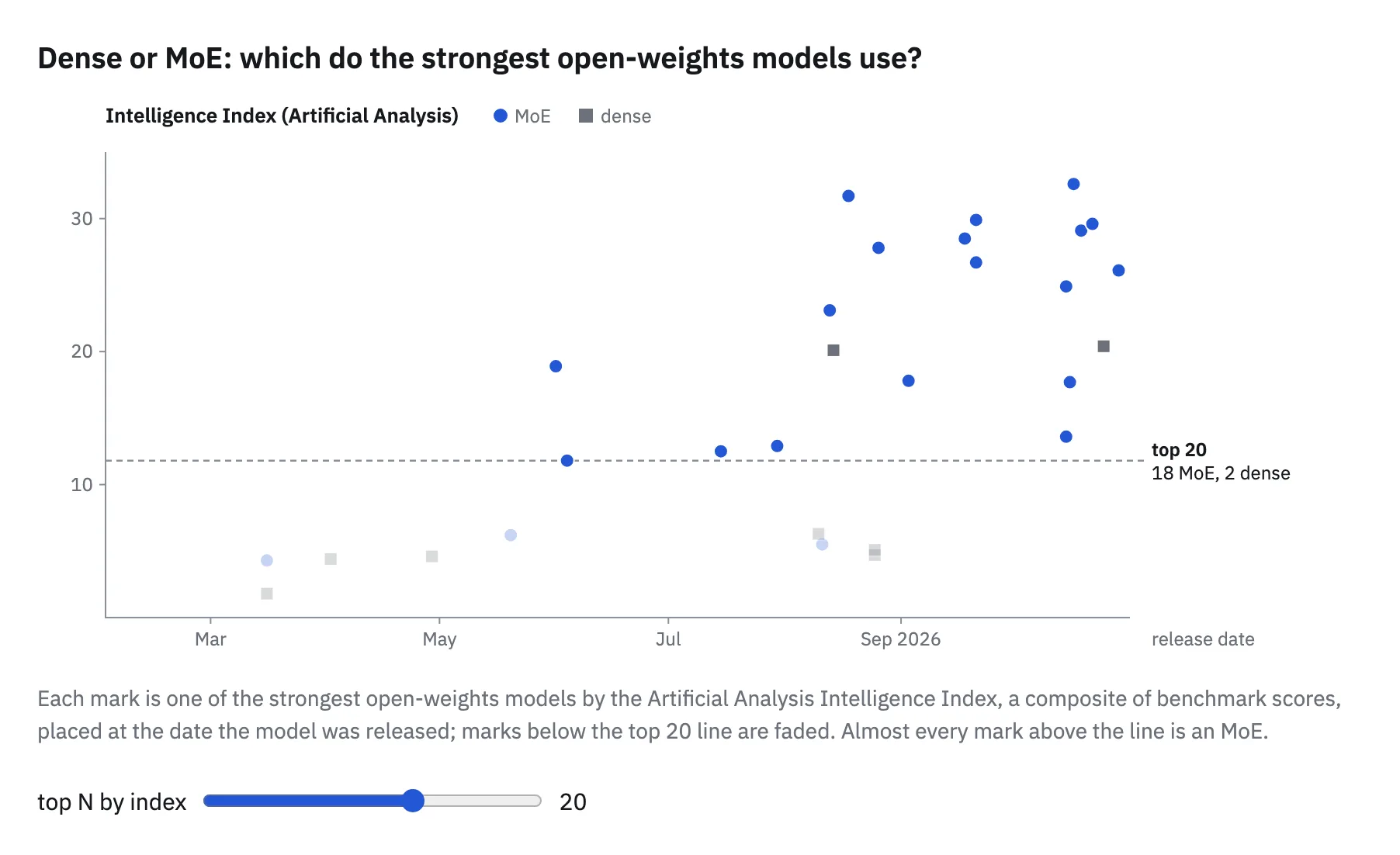
What an MoE offers lies in how it spends its inference compute. Each token runs through only a few of its experts, so the model can hold many more parameters than it uses on any one token: the small MoE you will train in chapter 2 has 6.86B parameters, of which 1.22B are active per token. Turning that inference saving into faster training is the hard part.
Our previous deep dive on training, the Smol Training Playbook, covered training a dense model but only touched on MoE design. Because the star of that book, SmolLM3, was a dense transformer, its training needed no technique specific to MoE, like expert parallelism. Still, we glanced at MoE in the playbook's "Going Sparse: MoE" section to cover its high-level design choices: sparsity, granularity, shared experts and load balancing. That section named the main reasons distributed MoE training is complex: expert placement, load balancing and all-to-all communication, but without diving into the particulars2. This handbook starts from that list.
Going from a dense model to an MoE gives you three new challenges to manage: a router that decides which experts each token uses, a load that has to stay balanced across the experts, and, once the experts are split across GPUs, an exchange of tokens between those GPUs in every MoE layer. Each aspect brings settings a dense run never had and new ways for a run to fail. The chapters that follow take those settings one at a time and examine them in detail, with code you can run and, in most cases, direct results and data from our own cluster experiments.
A run that goes south will give you a symptom but not the reason behind it. The map below is a high-level view to help you go back to the source: start from how a run fails, find the first signal of bad behavior (the canary in the coal mine), and go read the part of the post that explains the possible cause. You can keep this map at hand for the day a run goes wrong.

Now, before we start, a quick note on the intended audience. Who is this handbook for? You will benefit from it if you have trained a dense model on a GPU cluster and want to train an MoE next. Chapter 2 sets up what you need and has you train that small MoE on a single node. If you are more curious about how MoEs work and what frontier models choose than about running one, skip ahead to chapter 3, Anatomy of MoE Training.

Once the experts sit on different GPUs, every MoE layer exchanges tokens between them, a pattern our dense run never used. Can you trust your cluster's links with it before you change a single line of the model?
2. Setup and your first run
2.0 What you need
Every command in this chapter was written for one kind of machine, so that everyone runs the same environment: a Slurm cluster of eight-GPU nodes. This section describes that setup, how much of the post you can follow with one GPU or none, and how to rent an eight-GPU node on Hugging Face Jobs. If your machines differ, you can still follow the explanations and adapt the commands.
The cluster the commands assume
The commands expect a Slurm cluster whose GPU nodes hold eight GPUs each. Containers start through Enroot and Pyxis, which let srun launch a task inside an image.3,4 The per-node readiness check in 2.1 uses NVIDIA's DCGM diagnostics. Our runs used AWS P5 nodes connected by Elastic Fabric Adapter (EFA), each with eight H100 GPUs of 80 GB.
Most of the chapter fits on one node. The dense baseline and the first MoE each request a single node with eight GPUs of about 80 GB. Only the network checks need more: the all-to-all tests in 2.1 run on two, four and eight nodes, and the EFA image in 2.2 is verified on two.
The software comes from two pinned sources. The first is the NGC PyTorch image 26.06-py3, which 2.2 imports and extends with the cluster's network libraries. The second is a Megatron checkout at commit d6316eb45, which you mount into the container rather than build into it. You also need a filesystem that the CPU workers and the GPU nodes can both read, because 2.3 tokenizes the data on a CPU partition and the training jobs read the result from there.
Reading with one GPU, or none
You can get most of the post without a cluster. Chapter 3 takes the MoE layer apart: what each part does, what frontier models choose for it and the evidence behind each choice. You can read it end to end without running anything, and save its flags for when you have the hardware. Chapter 4 carries the same choices past pretraining, into serving and reinforcement learning.
In this chapter, the tokenization in 2.3 runs on CPUs. Its small sample runs on a single machine without Slurm, so you can produce and inspect the same files the training runs read. The training recipes in 2.4 and 2.5 assume eight GPUs of about 80 GB, and the MoE spreads its experts across all eight. With fewer GPUs, read them for the method: what stays fixed between the two runs, how the expert width is chosen and what to compare. The all-to-all tests in 2.1 and the EFA setup in 2.2 need several nodes to run as written.
Renting a node on Hugging Face Jobs
If you want to run the single-node parts without owning the hardware, Hugging Face Jobs runs a Docker image and a command on Hugging Face's machines, billed by the minute. It is open to any user or organization with a positive credit balance, and the monthly credits of a PRO, Team or Enterprise subscription can pay for jobs.5 The largest hardware options that hf jobs hardware lists have eight GPUs, as many as 2.4 and 2.5 use; h200x8, for example, holds eight H200s of 141 GB each.6
A job is defined by a Docker image from Docker Hub or a Hugging Face Space, a command and a hardware option, so running this chapter there means packaging the image from 2.2 as a Docker image and replacing the Slurm launcher with a Jobs command. A job stops after 30 minutes unless you set a different timeout.7 A first command only checks that the job sees all eight GPUs:
hf jobs run --flavor h200x8 --timeout 10m \
    pytorch/pytorch:2.6.0-cuda12.4-cudnn9-devel \
    python -c "import torch; print(torch.cuda.device_count())"
Whether you run the recipes on your own cluster or on a rented node, the machines you were given may not perform the way their specification says. How would you notice a GPU or a link that quietly underperforms?
2.1 Test your hardware
Before you start tuning a model, establish what the machines can do. With Megatron's alltoall dispatcher, each MoE layer sends tokens to the GPUs that hold their experts and returns the results through another all-to-all. The links between GPUs are therefore part of the work you need to test: a healthy all-reduce result alone does not tell you how quickly those token exchanges will run.
Run the checks below inside your job allocation, before launching training. With Pyxis, srun --container-image starts a container; the next section explains how to prepare the training image.3
Check each node
Start with a readiness check on every allocated node. NVIDIA's DCGM provides several diagnostic levels, with level 1 intended for readiness checks and the higher levels adding tests that help investigate failures. The command below runs one task per node so you can inspect each result before starting training.8
NNODES=$SLURM_JOB_NUM_NODES
srun --nodes="$NNODES" --ntasks="$NNODES" --ntasks-per-node=1 \
    dcgmi diag -r 1 --fail-early
If every node passes, proceed to the communication test. If a node fails, keep its diagnostic output and investigate it before proceeding. For example, a level 2 diagnostic reported thermal violations alongside failed PCIe and memory tests on three GPUs in one of our nodes.
Longer diagnostics belong in a separate maintenance window. NVIDIA describes levels 3 and 4 as administrator post-mortem tests, whereas level 1 is a readiness check.8
Prepare the diagnostic image
If your cluster already provides an nccl-tests image, set NCCL_TESTS_IMAGE to its path. Otherwise, on AWS with EFA you can import the public image maintained with the AWS NCCL test recipes. Choose a destination on a filesystem accessible to the allocated nodes:9
NCCL_TESTS_IMAGE=/shared/images/nccl-tests.sqsh
mkdir -p "$(dirname "$NCCL_TESTS_IMAGE")"
enroot import -o "$NCCL_TESTS_IMAGE" \
    'docker://public.ecr.aws#hpc-cloud/nccl-tests:latest'
Keep the imported SquashFS file with your baseline, since importing latest again can give you a different image. For a repeatable import, select a versioned tag from the AWS recipe in place of latest.10,9
The AWS recipe also provides a Dockerfile if you need to build the image. For another fabric, use its supported CUDA, NCCL, MPI and network-plugin stack; NVIDIA's nccl-tests build instructions explain how to select those library paths. Multi-node tests require a build with MPI=1. The benchmark below assumes that MPI can launch through Slurm's PMIx integration, so match the image to the cluster's MPI setup.11
Measure the collective you will use
Once the nodes pass, measure all-to-all bandwidth across the allocation. The command below launches one rank per GPU and exchanges an 8 GiB buffer per rank, matching the large-message test used for our baseline. Use the NCCL_TESTS_IMAGE path prepared above, adjusting the executable path if your image installs nccl-tests elsewhere.
srun --nodes="$NNODES" --ntasks="$((8 * NNODES))" \
    --ntasks-per-node=8 --gres=gpu:8 --mpi=pmix --cpu-bind=none \
    --container-image="$NCCL_TESTS_IMAGE" --no-container-mount-home \
    /opt/nccl-tests/build/alltoall_perf \
    -b 8G -e 8G -g 1 -c 1 -n 20
Check the rank listing before reading the result: an allocation of two eight-GPU nodes should list 16 ranks. Then inspect the busbw and #wrong columns for the tested size. Here is the out-of-place result from our two-node baseline, with the other columns omitted:
size (B)      busbw (GB/s)    #wrong
8589934592    77.14           0
The zero in #wrong means the correctness check passed for that result. The bandwidth gives you a reference for subsequent allocations with the same node count, GPUs per node and test settings. Keep the node list with it so that a later slow result can be traced back to the machines involved. In a separate two-node allocation, run with NCCL tuning variables set, the same message size reached 39.84 GB/s, so record which nodes and settings produced each baseline.
All-reduce remains useful as a comparison, but the two collectives can behave very differently on the same machines. That slower two-node test delivered 398.52 GB/s for all-reduce alongside its 39.84 GB/s all-to-all result. For an MoE that exchanges tokens across those nodes, the second measurement is the one that tests the relevant communication pattern.
Choose a baseline for each allocation size
As you add nodes, more of an all-to-all exchange crosses the inter-node network. Our multi-node sweep shows why the baseline must depend on node count: it reached 77.14 GB/s on two nodes, 39.25 GB/s on four, and 30.91 GB/s on eight. Compare each allocation with a baseline at its own node count, using the same message size and the same result column.
Before choosing a reference, repeat the check on a known-good configuration with the hardware, software and test settings held fixed. Use the resulting range to decide whether a new allocation is ready for training. A practical starting policy is to require 90% of the baseline bandwidth and a passing correctness check. With the two-node result above, the bandwidth threshold would be about 69 GB/s. Adjust the threshold to your cluster's observed variability. A fixed 33 GB/s threshold, for example, would accept the slow two-node result while rejecting the eight-node sweep result.
Keep this baseline unchanged while you investigate a slow allocation. If you also want to try NCCL tuning variables, compare the settings on the same nodes with the same test parameters. Our default and tuned runs used different node pairs, so their bandwidth difference cannot identify the effect of those variables.
Check for changes during training
For periodic hardware checks during training, use Megatron's --gpu-sniff-test-interval <n>. It runs before training and every n iterations (training.py#L4850-L4852, training.py#L4484-L4489), including an all-to-all over the expert-parallel group (gpu_sniff_test.py#L5-L21). Its outlier warnings identify ranks to investigate when a slowdown appears (gpu_sniff_test.py#L104-L118).
The diagnostic image has let you test the GPUs and their links. Your training image needs access to the same hardware, so let's prepare it and check its network libraries.
2.2 Build your image
A training environment has two parts to get right: the libraries that run GPU computations, and the network libraries that connect those GPUs across nodes. We start from an NVIDIA PyTorch container for the first part, then add the network support required by the cluster. Keeping Megatron in a separate checkout lets you change the training code while retaining the same image.
The examples here use Enroot and Pyxis on Slurm. The base image is NGC PyTorch 26.06-py3; the network-specific instructions apply to our AWS P5 nodes with EFA. On another cluster, use its supported network stack for that part of the image.3,4
Import the base image
Enroot imports a container image into a SquashFS file that Pyxis can launch through srun. Choose an output path accessible from your compute nodes, then import the base image:4
IMAGE=/path/to/images/pytorch-26.06.sqsh
enroot import -o "$IMAGE" docker://nvcr.io#nvidia/pytorch:26.06-py3
Keep the Megatron checkout outside this image and mount it into the container when you launch training. The flags in this post target commit d6316eb45; checking it out explicitly makes the code you read alongside the examples match the code you run. The source notes list the image and commit used for each measurement.
Put this checkout, and later the data and tokenizer, on a filesystem that both the CPU workers and GPU nodes can read. In the commands below, SHARED_ROOT is that directory and PROJECT_DIR is your project directory, with the companion scripts cloned into its scripts/ folder.
export SHARED_ROOT=/path/to/shared/work
export PROJECT_DIR="$SHARED_ROOT/moe-blogpost"
git clone https://gist.github.com/nmntz/5de952d686f66d7bce5bce8cba9d7139.git "$PROJECT_DIR/scripts"
git clone https://github.com/NVIDIA/Megatron-LM.git "$SHARED_ROOT/Megatron-LM"
cd "$SHARED_ROOT/Megatron-LM"
git checkout d6316eb45bf1bfbb6f1f848c0b56e55166564d80
Verify GPU access
Before adding the cluster's network libraries, check that the base image can import PyTorch and Transformer Engine and see the GPUs. Run this inside an allocated eight-GPU node, using the IMAGE path from above:
srun --nodes=1 --ntasks=1 --gres=gpu:8 \
    --container-image="$IMAGE" --no-container-mount-home \
    python -c '
import torch, transformer_engine
print("torch", torch.__version__)
print("transformer_engine", transformer_engine.__version__)
print("device_count", torch.cuda.device_count())
x = torch.randn(8).cuda().sum()
print("cuda sum ok", x.item())
'
The stock image reported the following versions and device count. The final line of the command also prints a sum computed on the GPU, so inspect that result along with the imports before proceeding.
torch 2.13.0a0+8145d630e8.nv26.06
transformer_engine 2.16.0+4220403e
device_count 8
The CUDA result checks execution on the GPU within this node. For EFA communication across nodes, add the network plugin and its dependencies described below.
Add EFA support
On our AWS nodes, the network layer consists of the EFA userspace libraries and the aws-ofi-nccl plugin built against the NCCL inside the image. The build used EFA installer 1.49.0 and aws-ofi-nccl v1.19.2. Record both versions alongside the base image in your build recipe.
The EFA image build script creates a writable Enroot container from the base image, installs the EFA userspace libraries with --skip-kmod, and compiles the plugin against the image's NCCL. It then exports a new SquashFS image and removes the temporary container. Run it on an allocated compute node with Enroot and GPU access, choosing a new output path:
EFA_IMAGE=/path/to/images/pytorch-26.06-efa.sqsh
bash "$PROJECT_DIR/scripts/build_efa_image.sh" "$IMAGE" "$EFA_IMAGE"
Use EFA_IMAGE as the --container-image path for subsequent training launches. The script prepares the network layer; keep the following environment settings with that image so the job can find and select its libraries.
Here, the library paths refer to the copies installed inside the container, and NCCL_NET_PLUGIN=ofi selects the plugin by name. Passing a filesystem path as the plugin value caused NCCL to construct an invalid library name in our setup.
export LD_LIBRARY_PATH=/opt/amazon/ofi-nccl/lib:/opt/amazon/efa/lib:${LD_LIBRARY_PATH:-}
export NCCL_NET_PLUGIN=ofi
export FI_PROVIDER=efa
export FI_EFA_USE_DEVICE_RDMA=1
export NCCL_SOCKET_IFNAME='^lo,docker0,veth_def_agent'
export NCCL_DEBUG=INFO
The socket interface exclusion addresses the initial connection NCCL uses to set up communication. On our nodes, NCCL selected veth_def_agent, tried to connect to its link-local address, and failed with Connection refused. Excluding that interface allowed the launch to proceed. Adapt the exclusion list to your cluster's interfaces before reusing it.
Verify the network path
On your first multi-node training launch, inspect the NCCL initialization log before interpreting training performance. This checks the network path from the training image itself. For the EFA image described here, the line to look for is:
NCCL INFO Using network LibfabricIf you see Using network Socket instead, read the plugin-loading messages immediately above it. An invalid plugin name or a missing library version can leave NCCL using sockets. For example, the EFA_1.4 error identifies a missing library version to resolve before trying again.
The log confirms which transport the job selected; measuring its bandwidth remains a separate check. Record the training image and network settings alongside the diagnostic result from 2.1, keeping the two environments explicit when comparing their performance.
With the hardware checked and the image prepared, we can turn to the first training run. It starts with the data: turning raw text into token sequences and storing them in the format Megatron expects.
2.3 Tokenize
Megatron reads training text from pairs of indexed files. The .bin file stores token IDs, while the .idx file tells the loader where each sequence begins and ends. Preparing these files once lets the dense and MoE runs read the same tokens, so changing the model does not also change the data.
We will use FineWeb-Edu and the Llama 3.2 tokenizer. Datatrove's MegatronDocumentTokenizer writes the format directly; the remaining work is to choose an output directory, check a small sample, and submit the larger tokenization job.
Prepare the tokenizer
Keep the data and tokenizer under SHARED_ROOT, the shared directory from 2.2. The tokenization script runs locally for the sample and submits a Slurm array for the larger job.
export TOKENIZER_DIR="$SHARED_ROOT/tokenizer"
python3.11 -m venv "$SHARED_ROOT/tokenize-venv"
source "$SHARED_ROOT/tokenize-venv/bin/activate"
python -m pip install \
    'datatrove @ git+https://github.com/huggingface/datatrove.git@2c895af7a95010a96fa53e2dc77cc0ce92799e3f' \
    pyarrow tokenizers huggingface_hub
The original tokenizer repository, meta-llama/Llama-3.2-1B, requires access approval. If your account has access, run hf auth login and use that repository in the download command. Otherwise, unsloth/Llama-3.2-1B provides an ungated copy: our comparison found matching vocabulary and token IDs. Both tokenization and training will read the same downloaded tokenizer files.12
TOKENIZER_REPO=unsloth/Llama-3.2-1B
hf download "$TOKENIZER_REPO" \
    --include 'tokenizer*' --include 'special_tokens_map.json' --include 'config.json' \
    --local-dir "$TOKENIZER_DIR"
Datatrove reads tokenizer.json from this directory and appends <|end_of_text|> after each document. Megatron later receives the directory through --tokenizer-model, which also gives it the tokenizer's configuration.
Check a small shard
Tokenize a small sample on a CPU compute node before submitting the full array. This command reads up to 1,000 documents and keeps them all, writing the result to a separate directory so the sample cannot be mistaken for the training corpus.
python "$PROJECT_DIR/scripts/tokenize_first_run.py" \
    --tokenizer "$TOKENIZER_DIR/tokenizer.json" \
    --output "$SHARED_ROOT/data-smoke" --limit 1000
The output prefix is fineweb-edu_00000_tokens. Check it with Megatron's own reader inside the training image from 2.2, using an allocation where Pyxis can launch the container. Deactivate the tokenization environment first so its Python does not override the image's interpreter. Set TRAIN_IMAGE to EFA_IMAGE on the EFA setup, or to the prepared training image for your cluster.
deactivate
export TRAIN_IMAGE="$EFA_IMAGE"
export MEGATRON_PATH="$SHARED_ROOT/Megatron-LM"
srun --nodes=1 --ntasks=1 \
    --container-image="$TRAIN_IMAGE" \
    --container-mounts="$SHARED_ROOT:$SHARED_ROOT" \
    --container-workdir="$MEGATRON_PATH" --no-container-mount-home \
    env PYTHONPATH="$MEGATRON_PATH" python -c '
import sys
from megatron.core.datasets.indexed_dataset import IndexedDataset
data = IndexedDataset(sys.argv[1])
assert len(data) > 0
print("sequences", len(data))
for i in range(min(3, len(data))):
    tokens = data[i]
    assert len(tokens) and tokens[-1] == 128001
    print("length", len(tokens), "last token", int(tokens[-1]))
' "$SHARED_ROOT/data-smoke/fineweb-edu_00000_tokens"
You should see a nonzero sequence count and last token 128001 for each inspected sequence. That final token is the document boundary we asked the tokenizer to append. Reading the shard through Megatron also checks that Megatron can parse the index and read the first sequences from the token file before GPU training starts.
Submit the tokenization job
The sample checks the file format; the larger job prepares a corpus to reuse as your training runs grow. Submit it from the login node with the same virtual environment activated. Set CPU_PARTITION to your cluster's CPU partition; add --qos if the scheduler requires one. The script requests 12 CPUs and 24 GB of memory per task, and the virtual environment must be accessible at the same path on those workers.
source "$SHARED_ROOT/tokenize-venv/bin/activate"
export OUT_DIR="$SHARED_ROOT/data/fineweb-edu"
CPU_PARTITION=your_cpu_partition
python "$PROJECT_DIR/scripts/tokenize_first_run.py" \
    --tokenizer "$TOKENIZER_DIR/tokenizer.json" --output "$OUT_DIR" \
    --tasks 100 --limit -1 --sample-rate 0.074 --partition "$CPU_PARTITION"
Datatrove prints the submitted job ID. Use that ID with squeue -j <job-id> to follow the array, and inspect failed tasks under $OUT_DIR/logs before relaunching the same command.
Each task reads a share of the input files and keeps a random 7.4% of the documents before tokenizing them. Because documents have different lengths, this fraction does not fix the number of tokens in the output. Keep the task count, sampling rate and output directory unchanged when restarting an interrupted job. Datatrove uses completion markers under the logging directory to skip finished tasks.13
Pass the shards to Megatron
Wait for the array to finish before building the training manifest. The following check requires all 100 task-completion markers and expected shard pairs and writes the shard prefixes to data-args.txt, one per line. Each prefix names both files, so neither .bin nor .idx belongs in the manifest.
export DATA_ARGS="$OUT_DIR/data-args.txt"
python - <<'PY'
import os
from pathlib import Path
root = Path(os.environ["OUT_DIR"])
prefixes = [root / f"fineweb-edu_{rank:05d}_tokens" for rank in range(100)]
for rank, prefix in enumerate(prefixes):
    assert (root / "logs/completions" / f"{rank:05d}").is_file(), rank
    for suffix in (".bin", ".idx"):
        path = Path(str(prefix) + suffix)
        assert path.is_file() and path.stat().st_size > 0, path
Path(os.environ["DATA_ARGS"]).write_text("\n".join(map(str, prefixes)) + "\n")
print(f"wrote {len(prefixes)} prefixes")
PY
deactivate
Training will read this file through --data-args-path. That option supplies the same list as --data-path, but keeps a long set of shards out of the launch command. The launcher also sets --data-cache-path to a persistent directory for Megatron's sample indices, allowing later runs with the same dataset configuration to reuse them.
For the first runs we use --split 100,0,0, assigning the data to training. Reserve a held-out split before using the run to compare model quality.
With a readable dataset and a manifest pointing to its shards, you can launch the dense baseline. Its loss, gradient norms and step times will establish a reference before we introduce experts.
2.4 Dense baseline
A dense run gives you something concrete to compare with when the MoE behaves unexpectedly. Both models will use the same data, batch size and optimizer, so a loss spike or a slow step can first be checked against the simpler model. This baseline also exercises the training image and data loader together before routing enters the picture.
The model has 16 transformer layers, a hidden size of 2,048 and an 8,192-wide feed-forward network. With the 128,256-entry vocabulary, it contains about 1.22 billion parameters. The recipe targets one node with eight GPUs with roughly 80 GB of memory each. We will reuse the launch script for the MoE.
Launch on one node
We will use Trackio to record the training metrics. Trackio is a lightweight, open-source experiment tracker from Hugging Face. Its API mirrors wandb, so import trackio as wandb is usually the only change existing code needs. Runs are logged to a local database you own, and you can browse them in a local dashboard or sync them to a Hugging Face Space to share live curves with your team, with no account or paid plan required.14
First, create a Python environment on shared storage from inside the training image. It inherits the image's GPU libraries and adds the pinned tracking package:
srun --nodes=1 --ntasks=1 \
    --container-image="$TRAIN_IMAGE" \
    --container-mounts="$SHARED_ROOT:$SHARED_ROOT" --no-container-mount-home \
    bash -c 'python -m venv --system-site-packages "$1/train-venv" &&
        "$1/train-venv/bin/python" -m pip install "trackio==0.42.0"' _ "$SHARED_ROOT"
export TRACKIO_PROJECT=moe-first-run
The launcher uses the Trackio entry point to send Megatron's scalar metrics to one run per job. Both runs share the project above, with their data stored under $SHARED_ROOT/trackio. The adapter uses Megatron's existing scalar-logging hooks, so flags such as --log-memory-to-tensorboard control which metrics reach Trackio.
The first-run script groups the training flags into Bash arrays. It uses the training image, pinned Megatron checkout, tokenizer directory and data manifest prepared in the previous sections. Keep the mounted paths under SHARED_ROOT and set TRAIN_IMAGE to the prepared SquashFS image.
From the shared blog checkout, submit the dense job to your GPU partition. Keep the variables from 2.3 exported when you submit the job. The script records the image path, Megatron commit and data manifest with its output.
cd "$PROJECT_DIR"
GPU_PARTITION=your_gpu_partition
sbatch --partition="$GPU_PARTITION" scripts/first_run.sbatch dense
Slurm reserves one eight-GPU node. Inside it, a single srun task starts torchrun, which launches one training process per GPU. Look for the run output under $SHARED_ROOT/runs/dense-<job-id> and the training log at first-run-<job-id>.out in the submission directory.
The initial run stops after 120 iterations. Checkpoint saving and validation are disabled for this setup check. Keep the log and Trackio data when you move on to the MoE; they are the reference for the next section.
To inspect the curves, run the dashboard on a machine that can read the saved directory, after installing trackio==0.42.0 there. Select the dense and MoE runs in the project to compare them.
TRACKIO_DIR="$SHARED_ROOT/trackio" trackio show --project "$TRACKIO_PROJECT"Understand the configuration
With tensor and pipeline parallelism both set to one, each GPU holds a copy of the dense model. Data parallelism distributes the batch across the eight GPUs, while the distributed optimizer and communication overlaps are enabled in both runs.
--tensor-model-parallel-size 1 --pipeline-model-parallel-size 1
--expert-model-parallel-size 1 --context-parallel-size 1
--use-distributed-optimizer --overlap-grad-reduce --overlap-param-gather
--micro-batch-size 8 --global-batch-size 512
A micro-batch contains eight sequences per GPU. Across eight GPUs, each micro-batch processes 64 sequences; eight gradient accumulation steps produce a global batch of 512. At a sequence length of 4,096, each optimizer step consumes 2,097,152 tokens. Keeping these quantities fixed will make dense and MoE step times directly comparable.
The learning rate follows a warmup, stable, decay schedule, selected by --lr-decay-style WSD. It warms up to 5e-4, holds that learning rate, then decays near the end of the configured token budget. The 120-iteration run ends during the stable phase; its stop condition does not shorten the learning-rate schedule.
Full activation recomputation keeps the starting configuration within the memory budget used for our baseline. With micro-batch size eight and the native cross-entropy implementation, the corresponding run without recomputation exhausted memory in the loss calculation. We keep recomputation in both models so that the first comparison does not mix a model change with a memory-saving change.
--recompute-granularity full --recompute-method uniform --recompute-num-layers 1
--cross-entropy-loss-fusion --cross-entropy-fusion-impl native
Keep the dense run's loss, gradient norm and step time in Trackio as your reference. When you replace the feed-forward layers with experts, these measurements will help you see how the change affects training.
2.5 Your first MoE
The dense model applies the same feed-forward network to every token. In the MoE, a router chooses eight of 64 smaller experts for each token, allowing the model to hold more parameters than it uses on any one token. We choose the expert width so that the eight selected experts contain the same number of feed-forward parameters as the dense layer they replace.
This gives us a 6.86-billion-parameter model with about 1.22 billion active parameters per token. The extra capacity comes with a new cost: the tokens have to reach their selected experts, and the expert outputs have to return to the processes that need them.

Replace the feed-forward layers
The launcher selects the MoE configuration when you pass moe. Submit it using the same exported paths and GPU partition as the dense run, keeping the image, checkout, tokenizer and data manifest unchanged:
sbatch --partition="$GPU_PARTITION" scripts/first_run.sbatch moeExpert parallelism increases from one to eight, distributing the 64 experts across the node's eight GPUs. Each GPU holds eight experts, while the router selects eight experts per token from the full set.
--expert-model-parallel-size 8 --expert-tensor-parallel-size 1
--num-experts 64 --moe-ffn-hidden-size 1024 --moe-router-topk 8
--moe-token-dispatcher-type alltoall --moe-grouped-gemm
--moe-router-load-balancing-type aux_loss --moe-aux-loss-coeff 1e-3
--moe-router-dtype fp32 --moe-per-layer-logging
alltoall moves the routed tokens between GPUs, and grouped GEMM executes the local experts' matrix multiplications. The auxiliary loss encourages the router to distribute work across experts, with a coefficient of 1e-3. We also compute router logits in fp32 and enable per-layer logging, giving us the initial settings and measurements that chapter 3 will examine.
Everything else stays in the common configuration, including full activation recomputation. In particular, the dense --ffn-hidden-size 8192 setting remains in the script, while --moe-ffn-hidden-size 1024 supplies the width of each expert.
Count active and total parameters
A bias-free SwiGLU expert has three weight matrices. With hidden size 2,048 and expert width 1,024, their combined size is 3 × 2048 × 1024 = 6,291,456 parameters. Selecting eight experts therefore uses 50,331,648 feed-forward parameters per token, matching the dense layer's 3 × 2048 × 8192 parameters.
All 64 experts together contain eight times as many feed-forward parameters. The whole model grows by a smaller factor because attention, embeddings and the other non-expert parameters stay the same size, and each layer gains a small router matrix. Summing those components across 16 layers gives 6.86 billion total parameters and 1.221 billion active parameters, compared with 1.219 billion in the dense model.
The result is about 5.6 times as many total parameters at nearly the same active parameter count. Matching active parameter counts does not guarantee equal step time: distributing tokens among experts changes how the GPU work is organized and introduces communication.
Keep a dense reference
An MoE with one expert and top-1 routing computes the same function as the dense model it came from, so it should train like it. In our run, a 1-expert MoE upcycled from a dense checkpoint and continued beside the dense run stayed within 0.00087 of it over 15 aligned steps. Start the MoE from its own initialization instead and the comparison says little, since the two runs sit 2.72 apart at iteration 4. The MoE side also logs a load-balancing loss of exactly 1 and about 32,770 zeros in its gradient against at most 17 for the dense run: the router weights, which get no gradient with a single expert. The parity run upcycles the dense checkpoint, a path 3.6 returns to.

At the pin, that upcycling path ran for us only with two local fixes to training.py. The first passes the dense model to the checkpoint loader under the keyword model (training.py#L3074-L3078), while load_checkpoint names that parameter ddp_model. The second concerns the dense model built for the load: the upcycling code switches the dense shape on in args (training.py#L3056-L3062), but the model builder reads the model configuration stored at startup (training.py#L2917-L2926), so that model keeps the MoE layer layout and the load stops on a missing pre_mlp_layernorm key.
Deterministic mode makes a run repeatable, so that a gap between two runs means something. At the pin, --deterministic-mode requires cross-entropy loss fusion, TP communication overlap and the fused aux-loss kernel to be off (determinism.py#L28-L37, determinism.py#L195-L210), and accepts NVTE_ALLOW_NONDETERMINISTIC_ALGO only at 0 (determinism.py#L85-L90); it sets NCCL_ALGO=Ring, NCCL_EP_HT_EM_AG_SCAN_MODE=1, NVTE_ALLOW_NONDETERMINISTIC_ALGO=0 and CUBLAS_WORKSPACE_CONFIG=:4096:8 itself when they are unset (determinism.py#L40-L50). The 2.4 launcher passes --cross-entropy-loss-fusion and exports NVTE_ALLOW_NONDETERMINISTIC_ALGO=1, so drop both before adding the flag. With these settings, two runs of this MoE shrunk to micro-batch 2, global batch 64 and 12 iterations printed the same lm loss, load-balancing loss, grad norm and gradient zeros at every iteration; without them the lm loss differed from the first iteration on, by up to 0.00063.
Switch on deterministic mode before you compare two runs or chase a NaN.
Keep the dense run and its configuration as a reference as you develop the MoE. Whenever a change makes training slower or the loss stops improving, return to the dense run in Trackio and compare step time, loss and gradient norm at the same batch size and sequence length. A problem that appears in both runs points you toward their shared setup; one that appears only in the MoE gives you a reason to investigate routing and expert execution.
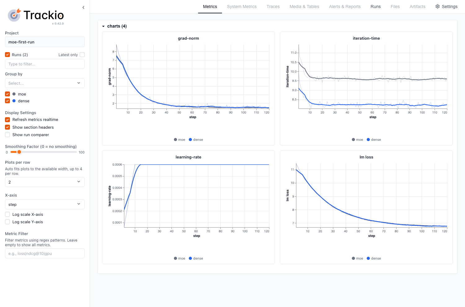
The dense reference helps you decide where to begin an investigation. Chapter 3 opens the MoE layer piece by piece, introducing the measurements you need to understand its behavior.
3. Anatomy of MoE Training
The MoE from 2.5 added parts the dense run never had: a router that picks eight experts for each token, experts that can end up with very different amounts of work, and an all-to-all that moves tokens between GPUs. Each of them can slow training or hurt the loss, and a gap against the dense reference does not, on its own, tell you which part caused it.
The figure below draws one MoE layer at a smaller scale than ours, with 16 experts and top-4 instead of 64 and top-8, plus a shared expert that ours does not have. It shows the tokens of a batch, the router, the experts and the sum that combines their outputs. Each section then opens on its own view of the same drawing, zoomed onto the part it covers, so you can skip to the part you need. A few views also carry a result from their section, such as the rogue experts that Step 3.5 Flash's training loss did not reveal (3.6)15.

After the monitoring setup in 3.0, we start inside the router, with how its scores become the weights of the chosen experts and whether tokens choose experts or experts choose tokens. Then come uneven load across experts, how many experts to use and how large, which layers get experts at all, and how to start a run and keep it stable. We end with where a training step spends its time on the GPUs.
3.0 Monitoring: turn it on once
Before changing any setting, turn on what tells you whether it worked. You do not need to know what every number means yet: each section introduces a metric when it first needs it (z-loss in 3.1, MaxVio in 3.2, timings and memory in 3.7). Appendix A.1 gives the capture commands, calculations and limits of each measurement.
What to turn on
The 2.5 run already logs the router losses per layer (--moe-per-layer-logging), so you can see which layer misbehaves (3.1, 3.3, A.1). Keep the Trackio launcher from 2.4 and add these flags to the 2.5 flags:
--save <dir> --save-interval <m>
--save-tokens-per-expert-interval <n>
--log-throughput --log-params-norm
--log-num-zeros-in-grad --log-max-attention-logit
Megatron writes the token counts and the activation dump below under --save (training.py#L3398-L3401) and asks for --save-interval beside it (arguments.py#L1321-L1323), so the run also saves checkpoints there. The next flag records how many tokens each expert received (3.3, A.1). The other four track the run's health: throughput, the parameter norm, the zeros in the gradient and the largest attention logit (3.6, A.1). The scalar metrics appear in the same Trackio project as your baseline, while routing captures stay in their own files. The NaN check is already on (arguments.py#L2825-L2827).
What to capture when you need it
Two more measurements are bounded captures: run them when a question calls for them.
The routing trace records which experts each token picked (3.1, 3.3, A.1). Its hooks on the routers do not fire under CUDA graph replay (router_trace.py#L23), and by default it traces every iteration (training_config.py#L363-L367), so turn graphs off and bound it:
--moe-routing-trace-path <dir> --moe-routing-trace-max-training-iters <n>
--cuda-graph-impl none
The activation dump saves the experts' activations under the same --save directory, so you can compute per-expert activation norms offline (3.4, A.1):
--save-activations-interval <n>With monitoring on, let's start where every token starts: the router. It picks the experts, but how much does each one count in the token's output?
3.1 Router scoring: how logits become weights
The router turns each token into one logit per expert, and in plain top-k routing the top-k logits pick the experts the token goes to. Between those logits and the weights that mix the experts' outputs sit four choices. The gating function, the output scale (a constant multiplied onto the weighted sum of the chosen experts' outputs) and the sharpness (how peaked the router's scores are, so how much the top expert dominates) change how much each chosen expert counts in the token's output, and how large that output is. In plain top-k routing, for a given token's logits, none of them changes which experts win: each keeps the experts in the same order, or applies after the top-k.
Precision is the exception. A bf16 router can round two close logits to the same value and so change the winners, which makes an fp32 router the one setting to always use here.
The table below shows what ten current open MoEs chose for each of the four, one row per model.
| Model | Gating function | Output scale | Sharpness | Router precision: in training; in inference code |
|---|---|---|---|---|
| DeepSeek-V4.1-Flash | sqrt(softplus) | renormalized, 1.5 at k = 6 (√k = 2.45) | a temperature setting, left at 1.016 | not stated; fp3216 |
| Gemma 4 26B-A4B | softmax | renormalized, then a learned per-expert scale, k = 8 of 128 (√k = 2.83)17 | normalized router input: RMSNorm, a learned scale and 1/√d17 | not stated; bf16, softmax in fp3217 |
| GLM-5.3 | sigmoid | renormalized, 2.5 at k = 8 (√k = 2.83) | none | not stated; fp3218 |
| Inkling | sigmoid, normalized jointly over the top-6 and its 2 shared experts19 | 8.0 times a learned global scale, over 6 routed plus 2 shared (√8 = 2.83)19 | none | not stated; bf1619 |
| Kimi K3 | sigmoid | renormalized, 1.0 at k = 16 of 896 (√k = 4)20 | none | above MXFP4 in post-training QAT21; fp3220 |
| MiMo-V2.6-Pro-RL | sigmoid | renormalized, no factor at k = 8 (√k = 2.83) | none | not stated; fp3222 |
| North-Mini-Code | sigmoid | not renormalized: the weights are the raw scores, k = 8 of 12823 | none | not stated; bf1623 |
| Qwen3.8-Flash-Next | softmax24 | renormalized, no factor at k = 10 (√k = 3.16)24 | none | not stated; bf16, softmax in fp3224 |
| Step-5-Preview | sigmoid25 | renormalized, 3.0 at k = 8 of 352 (√k = 2.83)25 | none | not stated; fp3225 |
| ZAYA1-8B | softmax over an MLP router's logits26 | not renormalized, top-1 of 16 plus a skip expert26 | none | softmax in fp32 during RL; bf1626 |
Let's start with the gating function. If it never changes the winners, what does it change?
Gating function
Softmax, sigmoid and sqrt(softplus) rank the experts the same way, so what differs is the weight each chosen expert gets. The figure below raises one token's logits from an unsure router to a confident one: softmax makes the top expert count more and more, while sigmoid saturates at large logits, so confident experts end up with equal weights. Gating functions keep the ranking when selection uses their scores alone. The expert bias of 3.3 is added to the gated scores before selection (moe_utils.py#L936-L938), so how far it moves an expert depends on the size of the scores, and a different gating function can change the top-k. Group-limited routing (3.7) can too, because it picks groups by summing their best scores (moe_utils.py#L712-L715).

In the figure, sqrt(softplus) lands between softmax and sigmoid: for positive logits, the ratio of two weights tends to the square root of the ratio of their logits as the scale grows. DeepSeek-V4 switched to sqrt(softplus) from sigmoid27. In Megatron, the expert bias of 3.3 needs sigmoid or sqrt(softplus): it refuses the bias with softmax at startup (transformer_config.py#L3139-L3147), and its softmax path never adds it. Wang et al., who proposed the bias28, explain why it fits softmax badly: softmax's normalization makes the gap between two experts depend on every other expert's score, so the bias is harder to tune. They still balanced a softmax router with it28. The auxiliary loss works with all three (moe_utils.py#L998-L1014).
Megatron source
moe_utils.py#L913-L927 (softmax, before or after top-k)
913if score_function == "softmax":914if use_pre_softmax:915scores = torch.softmax(logits, dim=-1, dtype=torch.float32)916if precomputed_indices is not None:917top_indices = precomputed_indices918probs = torch.gather(scores, dim=1, index=top_indices)919else:920probs, top_indices = compute_topk(scores, topk, num_groups, group_topk)921else:922if precomputed_indices is not None:923top_indices = precomputed_indices924scores = torch.gather(logits, dim=1, index=top_indices)925else:926scores, top_indices = compute_topk(logits, topk, num_groups, group_topk)927probs = torch.softmax(scores, dim=-1, dtype=torch.float32)
moe_utils.py#L928-L941
928elif score_function in ("sigmoid", "sqrtsoftplus"):929if score_function == "sigmoid":930scores = torch.sigmoid(logits.float())931else:932scores = torch.nn.functional.softplus(logits.float()).sqrt()933if precomputed_indices is not None:934top_indices = precomputed_indices935scores = torch.gather(scores, dim=1, index=top_indices)936elif expert_bias is not None:937scores_for_routing = scores + expert_bias.float()938_, top_indices = compute_topk(scores_for_routing, topk, num_groups, group_topk)939scores = torch.gather(scores, dim=1, index=top_indices)940else:941scores, top_indices = compute_topk(scores, topk, num_groups, group_topk)
(sigmoid, sqrt(softplus), bias only selects),
transformer_config.py#L3139-L3147 (the bias refused with softmax)
3139if self.moe_router_enable_expert_bias and self.moe_router_score_function not in (3140"sigmoid",3141"sqrtsoftplus",3142):3143raise ValueError(3144"Expert bias for aux-loss-free routing only supports 'sigmoid' and 'sqrtsoftplus' "3145"score functions. Please set --moe-router-score-function to 'sigmoid' or "3146"'sqrtsoftplus', or unset --moe-router-enable-expert-bias."3147)
Sigmoid gives the chosen experts equal weights once all their logits are large and positive, which is where the simulation's scaled-up token ends: a confident router with the flat gate that Sharpness returns to. To see whether a run's router gets there, record the routing trace with its logits on (A.1) and follow two numbers per layer: the top expert's weight, and the routing entropy, which is low when one expert takes most of the weight and high when the weights are spread.
Use sigmoid (or sqrt(softplus)) when you balance with the expert bias (3.3), since Megatron refuses the bias with softmax. Otherwise use softmax, Megatron's default.
The router's weights do two jobs. They pick the experts, and they are also the numbers that mix the experts' outputs: the layer returns each chosen expert's output times its weight, summed. The gating function decides how much each chosen expert counts against the others. It does not decide how much they count together: with softmax, the top-k weights sum to less than 1, by a different amount for each token, so the size of the layer's output moves with them. So how big should that combined output be?
Output scale
Two settings decide how big the experts' combined output is. The first is renormalization: rescale the k chosen weights so they sum to 1, and the output's size no longer moves with their sum. In Krajewski et al. renormalizing lowered validation loss from 2.219 to 2.183 at granularity 8Granularity 8: experts 8 times smaller, 8 times as many, and 8 times as many chosen per token, so parameters and compute stay the same; 3.4 compares granularities.29. Megatron renormalizes by default (moe_utils.py#L913-L942), and --moe-router-pre-softmax turns renormalization off. Softmax at top-1 requires that flag: with one expert chosen, softmax over its single logit is always 1, so the router gets no gradient (transformer_config.py#L3213-L3221).

The simulation sweeps toy tokens from an unsure router to a confident one, with uncorrelated experts of equal RMS: without renormalization the routed output's size follows the top-k probability mass, and renormalizing keeps it between 1/√k of one expert's RMS and one expert's RMS.
The second setting is the routed scaling factor, the constant multiplied onto the result. It is needed because, even renormalized, the size of the routed output depends on how much each expert counts. With all the weight on one expert, the output has that expert's root mean square (RMS). With equal weights on k uncorrelated experts of equal RMS, it drops to 1/√k of that, and a routed scaling factor near √k restores it. DeepSeek-V3 uses 2.5 at k = 830, and Kimi K2 2.827 ≈ √8. Shipped models disagree on its value: in the table above only GLM-5.3 and Step-5-Preview stay near √k, and Kimi went from √8 in K2 to 1.0 at k = 16 in K320. Scaling the routed output also changes its weight against the shared expert's output (3.4).
The figure's last row scales the expert's input instead of its output: Llama 4 sends each token to one expert and multiplies the token by that expert's sigmoid score before the expert runs31. Its SwiGLU experts have no biases, so the output shrinks roughly as the score squared, and the score also softens the SiLU gate.
Megatron source
moe_utils.py#L942-L947 (renormalize, then scale)
942probs = scores / (scores.sum(dim=-1, keepdim=True) + 1e-20) if topk > 1 else scores943else:944raise ValueError(f"Invalid score_function: {score_function}")945946if scaling_factor:947probs = probs * scaling_factor
transformer_config.py#L3213-L3221 (top-1 needs pre-softmax: softmax over one logit gives a zero gradient)
3213if (3214self.moe_router_topk == 13215and self.moe_router_score_function == "softmax"3216and not self.moe_router_pre_softmax3217and self.moe_router_load_balancing_type != "sinkhorn"3218):3219# Requires applying softmax before selecting the top-k when k is 1,3220# since softmax on a [num_tokens, 1] would yield a zero gradient.3221raise ValueError("Please use --moe-router-pre-softmax when topk is 1.")
Without renormalization, the size of the routed output follows the top-k probability mass from token to token, the setting that gave the higher loss above, so the number to watch is how large the routed output is for each token, the root of the sum of its squared weights. Compute it offline from the routing trace (A.1).
Keep renormalization on at top-k > 1, and use --moe-router-pre-softmax for softmax at top-1, or the router gets no gradient. The routed scaling factor has no settled value: √k restores the routed output's RMS only for equal weights on uncorrelated experts, and shipped models disagree on its value.
Both the weights and the output's size depend on how peaked the logits are. A router can get too sharp, with one expert taking all the weight, or too flat, averaging its top-k. What sets how peaked it is?
Sharpness
With softmax, a linear router gets sharper as the token's norm or the router's weights grow: the logits spread apart, and the top expert takes more of the weight. The figure below compares three ways to control that against the linear router. Logit soft-capping compresses mostly the logits near its cap. Normalizing the router input removes the part that comes from the token's norm. Gating logit normalization standardizes the logits across experts32, which sets their spread to a chosen scale.

The plain linear router in the figure sharpens as the token's norm or the router matrix grows, and soft-capping, which Grok 2 applies at 30 without renormalizing33, pulls the large-norm token's top weight back only once its logits near the cap. Normalizing the input, as Gemma 4 does17, routes both tokens alike but still sharpens as the matrix grows, and gating logit normalization is unaffected by both. Skywork-MoE used gating logit normalization against a gate so flat that the layer averages its top-k experts34. With it, training loss came out moderately lower35. Normalizing the router input was ablated only together with the expert embeddings36.
Megatron source
router.py#L1150-L1152 (jitter, then plain linear gate)
1150# Apply input jitter1151input = self.apply_input_jitter(input)1152logits = self.gating(input)
router.py#L824-L831 (multiplicative input jitter)
824if self.config.moe_input_jitter_eps is not None:825eps = self.config.moe_input_jitter_eps826if self.input_jitter is None:827self.input_jitter = torch.distributions.uniform.Uniform(828torch.tensor(1.0 - eps, dtype=input.dtype, device=input.device),829torch.tensor(1.0 + eps, dtype=input.dtype, device=input.device),830).rsample831return input * self.input_jitter(input.shape)
A flat gate, one that averages its top-k experts and makes the model learn worse, shows up as Max1/Max2, the top expert's weight over the second's, falling toward 1, as it did in Skywork-MoE without normalization35. Follow it per layer together with the top expert's weight, both from the routing trace (A.1).
If the gate goes flat, gating logit normalization fixed it in Skywork-MoE. On the router input, Megatron offers Switch-style multiplicative input jitter, --moe-input-jitter-eps.
Sharpness lives in the gaps between logits, and softmax ignores a shift shared by all of them. bf16 does not: if every logit drifts upward together, the values bf16 can represent get farther apart, and close experts can tie. Do those ties change which experts win?
Precision
Top-k orders tied experts in a way PyTorch does not specify37. The figure below simulates routing the same tokens with 64 experts and top-8 through a bf16 router, with and without z-loss, a penalty on the logits' logsumexp. Its simulated logits drift up by one shared offset, and it counts the tokens whose experts differ from what an fp32 router picks.

As the simulated offset rises, the bf16 router's logits land on a coarser grid and more tokens get different experts than under fp32. Z-loss lowers the logsumexp by pushing the logits negative. At top-8 of 64 the 8th logit sits about 3.5 below the logsumexp, so in the simulation it ends near −2.2 with z-loss and +3.6 without, two sizes bf16 rounds in steps of the same length, and about as many tokens change experts; only the fp32 router has no flips, since fp32 rounds 65,536 times more finely than bf1638. DeepSeek-V3.2, GLM-4.5 and Kimi K2.5 compute the router in fp32 in their inference code39. The case for fp32 rests on the training evidence, which is about stability. In Switch Transformers, a bf16 router diverged while an fp32 router trained at bf16 speed40. In ST-MoE, the router z-loss kept every run stable41. Labs rarely say what precision they train the router in: in the table above, 2 of the 10 reports mention it, and 5 of the 10 run the router's matrix multiply in bf16 in their inference code. How far below bf16 the rest of the layer can go, while the router keeps its precision, is the question 3.7 Precision returns to.
Megatron source
router.py#L124-L130 (router dtype)
124# Convert to specified datatype for routing computation if enabled125router_dtype = input.dtype126if self.config.moe_router_dtype == 'fp32':127router_dtype = torch.float32128elif self.config.moe_router_dtype == 'fp64':129router_dtype = torch.float64130logits = router_gating_linear(input, self.weight, self.bias, router_dtype)
moe_utils.py#L1424-L1435 (bf16 operands, fp32 logits)
1424if te_general_gemm is not None and router_dtype != torch.float64:1425# cuBLASLt's non-FP8 bias epilogue expects bias and output to have the same1426# dtype. Router parameters may be BF16 while router logits are FP32, so cast the1427# small bias vector before passing it to TE.1428gemm_bias = bias.to(router_dtype) if bias is not None else None1429output = te_general_gemm(weight, inp, router_dtype, layout="TN", bias=gemm_bias)[0]1430elif bias is None:1431output = torch.mm(inp.to(router_dtype), weight.to(router_dtype).t())1432else:1433output = torch.addmm(1434bias.to(router_dtype), inp.to(router_dtype), weight.to(router_dtype).t()1435)
moe_utils.py#L171-L184 (z-loss)
171logsum = torch.logsumexp(logits, dim=-1)172z_loss_values = torch.square(logsum)173174if padding_mask is not None:175# Invert padding_mask: True (padding) -> 0, False (valid) -> 1176valid_mask = ~padding_mask177# Only compute z_loss for valid (non-padding) tokens178z_loss_values = z_loss_values * valid_mask179# Compute mean over valid tokens only180num_valid_tokens = valid_mask.sum()181z_loss = z_loss_values.sum() / torch.clamp(num_valid_tokens, min=1.0) * z_loss_coeff182else:183z_loss = torch.mean(z_loss_values) * z_loss_coeff184return z_loss
router.py#L761-L764 (z-loss coefficient over TP×CP)
761if self.config.moe_z_loss_coeff is not None and self.training and torch.is_grad_enabled():762# Skip Z loss calculations when using torch.no_grad() or checkpointing.763moe_z_loss_coeff = self.config.moe_z_loss_coeff / self.tp_cp_group.size()764z_loss = z_loss_func(logits, moe_z_loss_coeff, padding_mask=padding_mask)
A bf16 router can make training diverge, as it did in Switch Transformers, so two signals are worth following: the z-loss, which tracks how far the logits drift up, and the flip rate, the share of tokens whose experts change when the router is recomputed in fp32. Megatron logs the z-loss when --moe-z-loss-coeff is set, already divided by the coefficient (router.py#L805-L807), so its square root is the RMS logsumexp: our run logged 20.9, an RMS logsumexp of about 4.6. The flip rate needs a matched capture of the same inputs and current router state; A.1 provides a bounded live hook, since the trace's initial weight snapshot does not track later training updates.
Always set --moe-router-dtype fp32. Add --moe-z-loss-coeff 1e-3, ST-MoE's value, to a softmax router whose logits drift up. DeepSeek-V3's report never mentions z-loss for its sigmoid router42.
What to watch
| Part | Symptom | Signal to watch |
|---|---|---|
| Gating function | The top expert's weight and the routing entropy, per layer, from the routing trace with logits on (A.1). | |
| Output scale | learns badly: without renormalization, the routed output scales with the top-k probability mass. Renormalizing lowered the loss29. | How large each token's routed output is, √(Σ w²), from the routing trace (A.1). |
| Sharpness | learns badly: when the gate is flat, the layer averages its top-k experts35. | The top expert's weight and Max1/Max2, its weight over the second expert's35, per layer, from the routing trace (A.1). |
| Precision | blows up: a bf16 router diverged in Switch Transformers40. | The logged z-loss is divided by its coefficient, so its square root gives RMS logsumexp: 20.9 corresponds to about 4.6. Measure fp32 routing flips with A.1's matched live hook using the same inputs and current router state; the trace's initial weight snapshot cannot replay later training forwards exactly. |
So far we have shaped how a token's logits become weights. The gating function sets how much each chosen expert counts, renormalization and the scaling factor set how big their combined output is, and sharpness and precision set how peaked and how exact the scores are. All of it assumed one setup: a learned router, and the token picking its top k. Both can change: experts can pick their tokens instead, and a fixed table can replace the learned choice. Who should make the choice, the token or the expert, and does the choice need to be learned at all?
3.2 Routing strategy: who selects, and how
Token-choice top-k is the default: each token scores every expert and keeps its k best. This section looks at two ways to change that. The expert can pick its tokens instead of the token picking its experts, or a fixed hash can pick, with no learned router at all.
| Model | Who selects | Token-id lookup |
|---|---|---|
| DeepSeek-V4-Pro | token choice | hash routing in the first 3 MoE layers44 |
| DeepSeek-V4.1-Flash | token choice | Engram n-gram memory (2- to 4-grams) at layers 1 and 14; no hash routing45 |
| EC-CF2 8B/64E (Zhou et al.)43 | expert choice | none |
| GLM-5.3 | token choice | none |
| Kimi K3 | token choice | none |
| Llama 4 Maverick | token choice | none46 |
| MiMo-V2.6-Pro-RL | token choice | none |
| Qwen3.8-Flash-Next | token choice | n-gram embedding (2- and 3-grams) at layer 147 |
| Step-5-Preview | token choice | none48 |
Before asking whether the choice needs a learned router, we have to settle who makes it, because with token choice many tokens can want the same experts and loads skew. Should each token keep picking its experts, or should each expert pick its tokens instead?
Who selects
With token choice, many tokens can want the same experts, so loads skew. Expert choice flips the roles: each expert takes its best tokens, so every expert gets the same load43. The catch is future token leakage49: whether a token gets an expert depends on the tokens after it. At inference those tokens do not exist yet, so routing differs from training50.
Expert threshold, the third rule in the figure below, keeps loads near even without looking at future tokens50. In exchange, each token gets a variable number of experts. In a 575M-parameter model it reached a lower loss than token choice, with or without balancing (2.844 against about 2.89)51.

In the figure, the sequence leans toward expert 1, and token choice, drawn with no balancer, overloads it. Expert choice balances the loads, but later tokens push out earlier selections, while expert threshold, whose cutoffs come from earlier batches that lean the same way, keeps the loads near the target without revising any selection, at the price of a varying number of experts per token.
Megatron source
moe_utils.py#L891-L897 (per-token top-k, token choice only)
891# Sorting top-k turned off during inference892return torch.topk(893scores,894k=topk,895dim=1,896sorted=torch.is_grad_enabled() or is_batch_invariant_mode_enabled(),897)
The skew token choice leaves behind makes the step slow. It shows in the token counts, tokens per expert per layer, which --save-tokens-per-expert-interval logs (A.1) and which read best as MaxVio, how far the busiest expert's load sits above the meanMaxVio, short for maximal violation: (busiest expert's load minus the mean load) divided by the mean load. 0 is perfectly even; 1 means the busiest expert gets twice the average. Wang et al., who proposed the expert bias of 3.3, define it.52.
Use token choice, the routing Megatron trains, with --moe-router-topk setting k.
Whether the token or the expert does the picking, the choice so far always comes from a learned router, so the routing itself has to be trained. Does routing really need to be learned, or could a simpler rule pick the experts?
Hash layers
In DeepSeek-V4's first 3 MoE layers, a fixed table maps each token id to its experts53, and the router is kept only for the weights54. The table is a fixed hash of the token id27, and in our probe it spreads frequent tokens no better than a random table. There is nothing to learn for the selection, and hash layers matched Switch and BASE layersLewis et al.'s balanced assignment of experts, which routes by solving a linear assignment that gives every expert an equal number of tokens. in models up to 4.5B55. The figure below puts learned and hash routing side by side, above a third lookup by token id: Engram, which hashes each token's last 2 to 4 tokens into tables of embeddings and adds the rows it reads to the hidden state56. DeepSeek-V4.1-Flash keeps Engram at two layers, but picks every layer's experts with its learned router57,58.

The figure's two routers treat the word "the" differently: the learned router selects each one by its context, while the hash layer sends every "the" to the six experts its table row names, even past an expert with a higher score. Both rows weight their six experts to sum to V4-Flash's routed scaling factor of 1.559, and the figure measures how alike the four "the"s' expert sets are by their mean Jaccard similarity. What the hash layer gives up is context: the same token id always selects the same experts, whatever surrounds it. It also scales worse than learned routing. Clark et al. varied how many of a model's layers are MoE layers. With a single MoE layer, hash routing reached the lowest loss of the routing methods they compared, but as more layers became MoE layers it stopped improving, while their learned router kept getting better60. And no bias can rebalance it54: frequent tokens can overload their assigned experts, and nothing moves them. V4.1-Flash dropped hash layers and kept only Engram, which picks no experts45.
In Megatron, --moe-num-hash-layers makes the first MoE layers hash layers (router.py#L304-L308). They read each token's experts from a token-to-expert table (tid2eid) with one row per vocabulary entry, and if you do not load one, Megatron fills it with a round-robin placeholder (router.py#L313-L329). Since the expert bias is off in these layers, nothing corrects a bad table during training, so the table matters. Roller et al. compared ways to build it: a random table and one that greedily spreads the most frequent tokens over the emptiest experts reached about the same perplexity, with the second better balanced, while grouping similar tokens by clustering their embeddings did clearly worse61.
Megatron source
router.py#L304-L308 (first N layers hashed)
304self.is_hash_layer = (305not self.is_mtp_layer306and hash_moe_layer_threshold > 0307and layer_number <= hash_moe_layer_threshold308)
router.py#L322-L326 (placeholder round-robin table)
322token_ids = torch.arange(self.config.hash_moe_vocab_size, device=self.weight.device)323expert_offsets = torch.arange(self.topk, device=token_ids.device)324self.tid2eid = ((token_ids[:, None] + expert_offsets) % self.num_experts).to(325torch.int32326)
router.py#L898-L905 (experts looked up by token id)
898flat_ids = input_ids.T.reshape(-1)899assert flat_ids.numel() == logits.shape[0], (900f"input_ids contains {flat_ids.numel()} tokens, but router logits contain "901f"{logits.shape[0]}."902)903# Token IDs address the real tokenizer vocabulary; reject out-of-range IDs,904# including negative IDs, without clamping them to another token's experts.905default_top_indices = self.tid2eid.index_select(0, flat_ids).long()
router.py#L914-L916 (weights still from the gate)
914def _compute_hash_topk(scores, topk, num_groups=None, group_topk=None):915del topk, num_groups, group_topk916return scores.gather(1, default_top_indices), default_top_indices
plus a few lines that load V4-Flash's layers.0.ffn.gate.tid2eid from the Hub and count tokens per expert
A table that overloads some experts makes the step slow, and since nothing rebalances it during training, check it early in the run by comparing the tokens per expert in the hash layers with those in the learned layers, from the token counts that --save-tokens-per-expert-interval writes (A.1).
Use it only to reproduce DeepSeek-V4's first layers. Load a fixed hash table as V4 does27, or a frequency-balanced one, instead of Megatron's round-robin placeholder.
What to watch
| Part | Symptom | Signal to watch |
|---|---|---|
| Who selects | slow: with token choice, some experts get more tokens than others. learns badly: with expert choice, routing at inference differs from routing in training. | MaxVio per layer52, how far the busiest expert's load sits above the mean, from the token counts (A.1). |
| Hash layers | slow: frequent tokens can overload the experts their hash assigns them, and no bias can move them. | Tokens per expert in the hash layers, compared with the learned layers, from the token counts (A.1). |
Expert choice and expert threshold keep the load even or close to it, and no bias can move a hash table's load. Megatron trains learned token choice, where nothing so far stops many tokens from crowding onto the same few experts. Crowded experts are the first real failure mode of an MoE, so how do we keep tokens spread evenly over the experts while the router keeps learning?
3.3 Load balancing
When many tokens pick the same experts, two things go wrong. The GPU holding the busiest experts has the most work, so the other GPUs wait for it and it sets the step time, and if the router keeps sending tokens to the same few experts, the others get few tokens and their parameters go mostly unused. The first cost is the easier one to measure: with routing forced even, the same model ran 1.5x faster at init.
Forcing the routing even only shows the speed to aim for, since it throws away what the router learned. To get close to it while the router keeps learning, there are two families of fixes, an auxiliary loss and a loss-free bias, and they balance the load in different ways. The aux loss adds a term that rewards an even load, so the router's gradient pushes its probabilities toward spreading tokens, at the price of a gradient that competes with the LM loss. The bias changes only which experts are selected. Whichever you pick, the scope it balances over (a sequence, a micro-batch or the global batch) decides what "balanced" means.
| Model | Auxiliary loss | Scope | Selection bias | Quantile balancing |
|---|---|---|---|---|
| DeepSeek-V362 | Small sequence-wise loss, coefficient 0.0001 | Batch-wide bias plus sequence-wise loss | Fixed-step expert bias | No, fixed-step updates |
| DeepSeek-V4.1-Flash63 | Small sequence-wise loss, coefficient 0.0001 | Text and image loads balanced separately, plus sequence-wise loss | Separate biases per modality, update speed 0.001 | Uses the auxiliary-loss-free bias strategy |
| Kimi K364 | Described as auxiliary-loss-free | Global batch | Bias derived from score margins, applied next step | Yes, global-batch histogram estimation |
| LongCat-Flash65 | Device-level balance loss | Global-batch FFN targets plus device-level balance within sequences | PID-controlled expert bias; identity experts excluded from bias updates | No, PID updates |
| MiMo-V2.6-Pro-RL66 | Router frozen during RL | Preserves the pre-RL router | Report evaluates freezing rather than a new bias update rule | No new balancing update reported for RL |
| Qwen3 MoE67 | Global-batch balancing loss | Global batch | No selection bias in the published router68 | No, auxiliary-loss approach |
Before comparing balancers, we need to know how much speed an uneven load costs us, since every balancer below should be judged against the throughput of routing that is forced to be even. Where does that 1.5x come from, and how do we measure it on our own setup?
Cost of imbalance
To see what imbalance costs, we routed the same model three ways. Forced-even routing, Megatron's --moe-router-force-load-balancing, replaces the router's logits with random ones so that every expert gets about the same load, which makes it the best case, at 149.4 TFLOP/s.
Forced-biased routing, --moe-router-force-biased, adds a shared random bias of growing size to those random logits, so a few experts get more and more of the tokens: a dial for how uneven the load is. At the far end of the dial throughput falls to 100.5 TFLOP/s, and a replay of that routing, whose aux loss matches the logged one, has the busiest expert receive every token, a MaxVio of 7, as uneven as top-8 routing over 64 experts can get. It can get worse: in the replay the busiest experts are spread over several GPUs, so the busiest GPU holds only about twice the mean load, and had they all sat on one GPU, that GPU would have done most of the expert work.
The learned router, the one you would train with, starts far from that best case: a freshly initialised router ran its first 40 iterations as slowly as the worst forced case. The figure below compares the three. Training has to close that gap without forcing the router's choices, and the rest of this section compares the balancing methods by how close they bring a learned router to forced-even throughput.

In the figure, throughput falls with each larger forced bias, as a few experts take more of the tokens, and the learned router starts at the level of the most uneven forced run. The busiest experts set the step because the all-to-all hands each GPU every token routed to its local experts, 8 of 64 in our runs, and the next all-to-all waits for the slowest GPU. A GPU's load is the sum over its local experts, so it can be more balanced than the per-expert load. That is why a balance loss can also work per GPU rather than per expert: DeepSeekMoE's device-level balance loss pools each GPU's experts into one term69, and the figure that follows compares it with the expert-level loss.

Trained on one toy batch with two experts per GPU, one of them among the four the LM favours, both losses balance the GPUs, and the device-level loss pulls the router less far from what the LM wants, since it sees only each GPU's total, which that placement keeps closer to even. The catch is that the experts within each GPU stay uneven, so one expert can still take most of its GPU's tokens. DeepSeekMoE gives the same reason for weighting the two losses unevenly: strict expert-level balance would cost model quality, so it sets a larger device-level factor and keeps a small expert-level one against routing collapse69. DeepSeek-V2 runs them at 0.05 against 0.00370. DeepSeek-V3's report no longer mentions a device-level loss: it balances each expert with a bias and a small sequence-wise loss, both covered later in this section42.
The same imbalance costs time in serving too, so a frontier MoE in production keeps it small: when DeepSeek serves DeepSeek-V4.1-Flash, its slowest GPU sits at most 1.09 times the mean71.
Megatron source
router.py#L1185-L1193 (force switches in forward)
1185if self.config.moe_router_force_load_balancing:1186# Apply force load balancing with random logits for benchmark1187logits = apply_random_logits(logits)11881189if self.config.moe_router_force_biased is not None:1190# Apply biased logits with shared random bias across all ranks1191logits = apply_biased_logits(1192logits, self.config.moe_router_force_biased, self.layer_number1193)
moe_utils.py#L1301-L1314 (random logits per rank)
1301@staticmethod1302def forward(ctx, logits: torch.Tensor) -> torch.Tensor:1303"""1304Forward pass returns random logits with rank-specific seed.13051306Args:1307logits (torch.Tensor): The logits.13081309Returns:1310torch.Tensor: The random logits.1311"""1312with get_cuda_rng_tracker().fork(get_expert_parallel_rng_tracker_name()):1313random_logits = logits.clone().normal_()1314return random_logits
moe_utils.py#L1353-L1370 (shared per-layer bias)
1353@staticmethod1354def forward(ctx, logits, std, layer_number):1355"""Forward pass: apply random bias to logits."""1356# Check cache if reuse mode (negative std)1357if std < 0 and layer_number in RandomSTEShared._cache:1358return logits + RandomSTEShared._cache[layer_number]13591360# Generate random bias with shared seed across all ranks1361with get_cuda_rng_tracker().fork(get_data_parallel_rng_tracker_name()):1362bias = torch.empty(logits.shape[-1], device=logits.device, dtype=logits.dtype).normal_(1363std=abs(std)1364)13651366# Cache if reuse mode1367if std < 0 and layer_number is not None:1368RandomSTEShared._cache[layer_number] = bias13691370return logits + bias
Imbalance shows up as a slow step, so the number to watch is TFLOP/s against the forced-even control run. To see where the lost time goes, look at the step profiled in 3.7: it ran on an unbalanced router, and 3.7 shows how to tell whether imbalance is what slows its all-to-all.
Use it once per setup, as a control run: --moe-router-force-load-balancing gives the balanced throughput to compare every balancer against. Never train with it.
Forced routing shows how fast an even load runs, but it replaces the router's logits with random ones, so it can only serve as a control run, never as a way to train. How do we steer a learned router toward an even load while it trains, starting with the oldest fix, a loss term?
Aux loss
The oldest fix adds a loss term, the aux loss: the coefficient times the expert count times a sum over experts, each expert's share of the micro-batch's tokens times its mean router probability (moe_utils.py#L148-L152). Its gradient pulls router probabilities away from what the LM wants, toward an even load. Below, four settings route one batch: no balancing, the aux loss at a small and at a large coefficient, and the loss-free bias.

Both balancers spread the load in the figure, in different ways: the aux loss pulls the router's probabilities off what the LM loss wants, further at the larger coefficient, while the loss-free bias only changes which experts are picked and balances best, though it reroutes the most selections. The aux loss's pull makes its coefficient a tradeoff: too large a coefficient costs LM loss, and too small a coefficient leaves the load uneven. Yuan3.0's ablation of DeepSeek-V3's sequence-wise aux loss on a 10B model, plotted in the next figure, shows both sides: test loss rose with the coefficient from 1e-3 to 0.1, while the smallest coefficient, 1e-4, did slightly better than no aux loss at all but still left the busiest expert in a layer with about 13.6 times the tokens of the least used one72,73.

The smallest coefficient in the figure leaves the load uneven, and the one that balances it, 1e-2, raises the test loss. Megatron sets the coefficient with --moe-aux-loss-coeff next to --moe-router-load-balancing-type aux_loss, one coefficient per loss type, applied in every layer. Motif 3 found its first MoE layers more susceptible to imbalance and gives them stronger auxiliary loss weights74. We come back to the first layers later in the chapter.
Megatron source
moe_utils.py#L148-L152 (Σ f·P times coefficient)
148aggregated_probs_per_expert = probs.sum(dim=0)149aux_loss = torch.sum(aggregated_probs_per_expert * tokens_per_expert) * (150num_experts * moe_aux_loss_coeff / (topk * total_num_tokens * total_num_tokens)151)152return aux_loss
router.py#L515-L536 (counts over one micro-batch)
515aux_loss_coeff = self.get_aux_loss_coeff("aux_loss")516if aux_loss_coeff == 0:517return probs518519global_tokens_per_expert, local_num_tokens, total_num_tokens = (520get_tokens_per_expert_and_token_count(521routing_map=routing_map,522reduce_group=self.tp_cp_group,523topk=self.topk,524with_padding_mask=with_padding_mask,525)526)527528aux_loss = switch_load_balancing_loss_func(529probs=scores_for_aux_loss,530tokens_per_expert=global_tokens_per_expert,531total_num_tokens=total_num_tokens,532topk=self.topk,533num_experts=self.config.num_moe_experts,534moe_aux_loss_coeff=aux_loss_coeff,535fused=self.config.moe_router_aux_loss_fusion,536)
router.py#L459-L472 (coefficient per loss type)
459def get_aux_loss_coeff(self, aux_loss_type: str) -> float:460"""Return the aux loss coeff for the given auxiliary loss type.461If the auxiliary loss type is not found, return 0.0.462"""463if isinstance(self.routing_type, str):464if self.routing_type == aux_loss_type:465return self.config.moe_aux_loss_coeff466if isinstance(self.routing_type, list):467try:468idx = self.routing_type.index(aux_loss_type)469return self.config.moe_aux_loss_coeff[idx]470except ValueError:471return 0.0472return 0.0
The measured row under the four-column figure above comes from Wang et al., who proposed the loss-free bias and compared it with a per-sequence aux loss on a 1B MoE with 64 routed experts and top-6. At their baseline coefficient of 1e-3, MaxVio over the validation set was 0.72 at a perplexity of 9.56, against 0.04 and 9.50 with the bias75; with no aux loss MaxVio rose to about 5.1, and at 1e-2 it fell to about 0.1 while perplexity rose to about 9.6976.
This aux loss, at a coefficient of 1e-3, is the learned router of Cost of imbalance, and by the end of its 120 iterations it had climbed to 125 TFLOP/s.
A coefficient set too high makes the model learn worse, and one set too low leaves the load uneven, so watch the LM loss and the balance together. Balance is best read from MaxVio rather than from the aux loss itself. The loss multiplies each expert's share of the tokens by its mean router probability, so when the router's probabilities are flat the loss reads the same as for an even load, whatever the token shares are, and a perfectly balanced reading can hide a skewed load. Sigma-MoE-Tiny hit this case: in its lower layers the loss went to its minimum by flattening the probabilities while the load stayed uneven77. --moe-per-layer-logging logs this value per layer as load_balancing_loss, divided by the coefficient.
Use it when the simplest balancer will do: aux_loss at a coefficient around 1e-3, as in our first MoE run in 2.5. Raise it if the load stays uneven, lower it if the LM loss suffers72.
The aux loss we used so far counts each expert's load within one micro-batch, which leaves a question we have not asked yet: over which tokens should the load be even? You could balance it over each sequence, over each micro-batch, or over the whole global batch, and the next part compares the three.
Scope
Think about what one micro-batch holds. Pretraining pipelines often pack each micro-batch from a single domain, say all code, so a loss that asks for an even load inside that micro-batch spreads the code tokens over every expert, and no expert gets to specialize in code78. Balance over the whole global batch instead, which mixes many domains, and the code tokens may crowd onto a few experts as long as tokens from other domains fill the rest. Qiu et al. saw experts specialize by domain only in that second setting, and it also lowered their perplexity79. The GPUs pay for it: inside each micro-batch the load is no longer even, and their 43B model's step ran about 6% slower, about 1% of that slowdown from communication overhead and the rest mainly from the uneven load80,81.
A single sequence is the tightest scope of all. Balancing each sequence on its own spreads every sequence over all the experts, even when a micro-batch mixes domains; DeepSeek-V2-Lite counted its only balance loss, an expert-level one, this way82, and DeepSeek-V3 keeps a small one to stop a single sequence from piling onto a few experts while the batch as a whole looks balanced42. In the figure below the three scopes run side by side, on GPUs that each hold two sequences from two domains: the tighter the scope, the less the experts can concentrate on one domain, and the looser it is, the more uneven the load each GPU carries.

In that simulation, the sequence-wise loss spreads the code sequence over all the experts, the micro-batch loss lets each GPU's two domains split its experts between them, and the global-batch loss leaves the code tokens mostly on their two favoured experts, at the price of the most uneven load per GPU. Megatron picks the scope through the load-balancing type: aux_loss balances per micro-batch, seq_aux_loss per sequence and global_aux_loss over the global batch. To combine scopes, pass several types and one coefficient for each, in the same order, for example --moe-router-load-balancing-type aux_loss seq_aux_loss --moe-aux-loss-coeff 1e-3 1e-4.
Megatron source
router.py#L567-L589 (per-sequence counts, ÷ bsz)
567scores_for_aux_loss = scores_for_aux_loss.reshape(seq_length, -1)568routing_map = routing_map.reshape(seq_length, -1)569570global_tokens_per_expert, local_num_tokens, total_num_tokens = (571get_tokens_per_expert_and_token_count(572routing_map=routing_map,573reduce_group=self.tp_cp_group,574with_padding_mask=with_padding_mask,575topk=self.topk * bsz,576)577)578579aux_loss = (580switch_load_balancing_loss_func(581probs=scores_for_aux_loss,582tokens_per_expert=global_tokens_per_expert,583total_num_tokens=total_num_tokens,584topk=self.topk,585num_experts=self.config.num_moe_experts,586moe_aux_loss_coeff=seq_aux_loss_coeff,587fused=self.config.moe_router_aux_loss_fusion,588)589/ bsz
router.py#L617-L628 (global counts, running average)
617global_tokens_per_expert, local_num_tokens, total_num_tokens = (618get_tokens_per_expert_and_token_count(619routing_map=routing_map,620reduce_group=self.tp_dp_cp_group,621with_padding_mask=with_padding_mask,622topk=self.topk,623)624)625626self.global_tokens_per_expert += global_tokens_per_expert627self.ga_steps += 1628averated_tokens_per_expert = self.global_tokens_per_expert / self.ga_steps
router.py#L233-L248 (global count buffers)
233# Initialize global tokens per expert for global aux loss234if self.get_aux_loss_coeff("global_aux_loss") > 0:235self.register_buffer(236'global_tokens_per_expert',237torch.zeros(238self.config.num_moe_experts,239dtype=torch.float32,240device=torch.cuda.current_device(),241),242persistent=False,243)244self.register_buffer(245'ga_steps',246torch.tensor(0, dtype=torch.float32, device=torch.cuda.current_device()),247persistent=False,248)
router.py#L1121-L1125 (reset per global batch)
1121def reset_global_aux_loss_tracker(self):1122"""Reset the global aux loss tracker."""1123if self.global_tokens_per_expert is not None:1124self.global_tokens_per_expert.zero_()1125self.ga_steps.zero_()
Each scope fails in its own way. Balancing per sequence or per micro-batch can keep domain experts from forming, so the model learns worse, while balancing over the global batch leaves the load on each GPU uneven, so the step gets slower. Whichever scope you pick, read balance from MaxVio at that scope, computed per micro-batch from the loads --save-tokens-per-expert-interval saves, per global batch from the sum of those loads, and per sequence offline from the routing trace (A.1).
Use micro-batch (aux_loss) by default. Use global_aux_loss only for domain-specialized experts, at +5.8% step time in Qiu et al.81.
Whichever scope you pick, a balancing loss still steers the router through its gradient, and that gradient competes with the one from the LM loss. Could you balance the load without touching the gradient at all?
Loss-free bias
The aux loss fixes an overloaded expert by pulling the router's probabilities away from what the LM wants. The loss-free bias leaves the probabilities alone and moves the load with no gradient. Each expert gets a bias, added to its score before the top-k and used only to pick experts, while the weights still come from the scores, and once per step Megatron moves each bias by a fixed amount, the update rate: up for underloaded experts, down for overloaded ones. The next figure runs that loop. In DeepSeek-V3's ablation it matched a batch-wise aux loss in validation loss, at 1B and at 3B83. Like the aux loss, it reroutes some selections away from the LM's own top-k, and in the four-column toy of the Aux loss part it reroutes the most.

The figure runs 16 toy experts with a step far larger than Megatron's default, so a few rounds stand in for many: overloaded experts lower their bias and underloaded ones raise it until the load is close to even, and the back-and-forth that the large step leaves is damped once the toy cuts its step tenfold. In real training the catch is the fixed step, which must suit the expert count. Li et al. swept the expert count of small MoEs, and with an update rate of 1e-3 the busiest expert's load grew with it, to about 50 times the mean at 1,024 experts, where an aux loss of 1e-2 alone stayed under about 7 times84. Above 128 experts the bias also hurt LM quality, and the authors suspect a step too coarse for that many experts85.
The reference lines on the overload trace in the figure above come from the same 1B runs, measured on each training batch rather than over the validation set: MaxVio settled near 0.72 with the aux loss at 1e-3 and near 0.1 with the bias86.
Megatron's rule is the simplest one you could write: every step, each bias moves up or down by the same fixed amount, however far its expert sits from the mean load. That is the sign update, and it is not the only way to run the loop. A linear update moves each bias in proportion to its expert's distance from the mean load, so a badly overloaded expert gets a large correction and a nearly balanced one a small one, while an AdamW update adapts the step for each expert. LongCat-Flash runs a linear update, aimed at the expert loads its compute budget calls for65, and ZAYA1-8B feeds each expert's load error to AdamW87.
The rules also differ in a subtler way: when an update's steps do not sum to zero, the mean of all the biases drifts. That drift changes no selection, since adding the same number to every expert's score leaves the top-k as it was, but it costs precision where the bias is stored in bf16; Megatron keeps it in fp32. Moonlight and Trinity Mini avoid the drift by subtracting the mean of the steps88,89. The released weights differ the same way: DeepSeek-V3's biases sit at a per-layer mean of 2.2 to 8.0, while Moonlight's and ZAYA1-8B's average 0 and LongCat-Flash's sit just below it90. Below, the sign update, a centered sign update, the linear update and the AdamW update run on the same batch.

The figure's toy batch has a few hot experts and many just under the mean load, so most sign steps point up: the sign and AdamW updates lift the mean of the biases while the centered sign and linear updates keep it at zero, yet the sign update balances as well as the centered one at every step, since top-k ignores a shift shared by all experts. Whatever rule moves it, the bias can only balance the tokens it counts. A batch-wide bias is fitted on one batch and applied to the next, so it can make the batch as a whole look even without guaranteeing that each sequence is: a single sequence can still pile onto a few experts. The obvious fix, a second bias computed over each whole sequence, would use tokens that come later in that sequence, and so leak the future into the routing of the earlier ones.
Chang's causal bias avoids the leak by building that second bias only from what the sequence has already routed. It resets at the start of every sequence, and after each token it lowers the bias of the experts just picked and raises the others', so each expert's bias tracks how far its picks so far sit above or below its share, k/N per token, and an expert this sequence has overused is pushed down for the tokens that follow. Like the batch bias, it only changes which experts are picked and is never trained by the gradient91. The next figure routes the same sequence with the global-batch bias alone and with the causal bias from this sequence's past added on top.

The sequence shown switches to code halfway. With only the global-batch bias, its code tokens pile onto one expert, even though the whole batch stays balanced; with the causal bias added, those code tokens spread over more experts and the sequence's load stays much closer to even. On the other hand, the simulation shows the causal bias sending more of the picks to experts outside the router's own top-k, away from what the router itself prefers, and the evidence for it is small-scale, from Chang's experiments on nanochat and TinyStories91.
Released models handle the single sequence differently. DeepSeek-V3 pairs its bias with the sequence-wise aux loss we saw earlier, at a tiny coefficient of 1e-462: the bias keeps the batch even, and the small loss guards against extreme imbalance within a single sequence. The figure that follows compares no such loss, a small one and a large one, on an ordinary sequence and on an extreme one.

In that toy, whose two coefficients are illustrative rather than DeepSeek-V3's, a small coefficient brings an ordinary sequence closer to even while moving the router only a little, but leaves an extreme sequence piled onto one expert; spreading that one takes a large coefficient, which pulls the router much further off the routing the LM loss prefers. A sequence is one way a batch-wide count can hide an imbalance, and a modality is another.
When a batch mixes modalities, a bias counted over all the tokens can balance their sum while the tokens of one modality, taken alone, still crowd onto a few experts. DeepSeek-VL2 and Kimi-VL keep one bias for all tokens92,93, and DeepSeek-V4.1-Flash keeps one per modality63. The figure below compares one shared bias with one bias per modality, each counting only its own modality's tokens.

The toy scripts text to lean toward four of its eight experts and images toward the other four, so a shared bias balances the total while each modality's surplus cancels the other's, and a bias per modality balances each modality on its own. The price of the split is that the bias then pushes every expert to take its share of each modality, away from specializing in images.
To run it in Megatron, turn the bias on with --moe-router-enable-expert-bias and set its fixed step with --moe-router-bias-update-rate, with sigmoid scores (--moe-router-score-function sigmoid), since Megatron accepts the bias only with sigmoid or sqrt(softplus) scores (transformer_config.py#L3139-L3147).
Megatron source
moe_utils.py#L936-L939 (bias in selection only)
936elif expert_bias is not None:937scores_for_routing = scores + expert_bias.float()938_, top_indices = compute_topk(scores_for_routing, topk, num_groups, group_topk)939scores = torch.gather(scores, dim=1, index=top_indices)
router.py#L209-L228 (int64 counts, fp32 bias)
209if self.enable_expert_bias:210self.register_buffer(211'local_tokens_per_expert',212torch.zeros(213self.config.num_moe_experts,214# Keep token counts exact through accumulation and cross-rank reduction.215# Float16Module leaves integer buffers in their original dtype.216dtype=torch.int64,217device=torch.cuda.current_device(),218),219persistent=False,220)221self.register_buffer(222'expert_bias',223torch.zeros(224self.config.num_moe_experts,225dtype=torch.float32,226device=torch.cuda.current_device(),227),228)
moe_utils.py#L1253-L1263 (sign update, exact compare)
1253# All Reduce Across TPxCPxDP group1254torch.distributed.all_reduce(tokens_per_expert, group=tp_dp_cp_group)1255num_experts = tokens_per_expert.shape[-1]1256total_tokens = tokens_per_expert.sum(dim=-1, keepdim=True)1257# Compare each tokens_per_expert value with the row average without converting the integer1258# counts to floating point: tokens_per_expert < total / num_experts iff1259# tokens_per_expert * num_experts < total.1260update_direction = torch.sign(total_tokens - tokens_per_expert * num_experts)1261updated_expert_bias = (1262expert_bias + update_direction.to(dtype=expert_bias.dtype) * expert_bias_update_rate1263)
finalize_model_grads.py#L726-L731 (update once per step)
726if config.moe_router_enable_expert_bias:727if pg_collection is None:728tp_dp_cp_group = parallel_state.get_tensor_and_data_parallel_group(729with_context_parallel=True730)731_update_router_expert_bias(model, config, tp_dp_cp_group=tp_dp_cp_group)
When the update rate is too coarse for your expert count, the load stays uneven, which slows the step as Cost of imbalance showed, and above 128 experts Li et al.'s sweep also saw LM quality suffer. You can catch it in two places. Every checkpoint saves expert_bias, so you can follow how far the biases of each layer spread from one checkpoint to the next, and the token counts that --save-tokens-per-expert-interval writes give you MaxVio per global batch (A.1).
Use it when the balancer must barely pull against the LM loss: the bias adds no gradient at all, and DeepSeek-V3's sequence-wise loss at α = 1e-462 adds very little. Run it with sigmoid scores, and tune the update rate to your expert count, since 1e-3 can be too coarse above 128 experts85.
The bias moves by the same small step whatever the load looks like, so it can take many steps to catch up with a router that keeps changing. Instead of stepping toward the right bias, could you compute it directly from the scores of the current batch?
Quantile
Quantile balancing keeps the bias but solves for it. For each expert, it ranks the micro-batch's tokens by their score for that expert and reads off a quantile: the score that only the expert's target share of tokens beats. The bias is set from that quantile instead of moved by a fixed step. Jin et al. compared balancers on a 19B-parameter MoE with 768 experts, and quantile balancing balanced sooner than the sign update at about the same LM loss, halving the average MaxVio, though over the last 1k steps its MaxVio ended slightly higher94. That precision has a price: in every micro-batch, each expert has to rank all of the micro-batch's tokens by its score to find its quantile, a top-k per expert on top of the usual top-k per token. Side by side below, the sign update and quantile balancing run on the same batch.

The toy routes the same batch at every step, so each solved bias routes the very tokens it was solved from: after the last step the sign update still leaves the load uneven, while quantile balancing brings it close to even within a few steps. In Megatron, each micro-batch solves for its own quantiles, and the solutions are averaged over the global batch to route the next one, optionally smoothed by an exponential moving average (EMA, --moe-router-quantile-balancing-ema).An EMA keeps most of the previous bias and mixes in only a share of each new solution, so the bias changes slowly from step to step.
Megatron source
moe_utils.py#L233-L247 (top-k and per-expert quantile)
233topk_result = (scores - beta).topk(k + 1, dim=1)234indices = topk_result.indices[:, :-1]235236if not update_beta:237return indices, beta238239assert (num_tokens * k) % num_experts == 0, (240"Quantile balancing requires the number of routed assignments "241f"({num_tokens} tokens * top-{k}) to be divisible by "242f"{num_experts} experts."243)244col_target = num_tokens * k // num_experts245alpha = topk_result.values[:, -1:]246beta_local = (scores - alpha).topk(col_target + 1, dim=0).values[-1].contiguous()247return indices, beta_local
finalize_model_grads.py#L441-L457 (average, EMA, re-center)
441stacked_beta = torch.stack(qb_beta_list, dim=0)442local_avg_list = [443accum / count.clamp(min=1).to(accum.dtype)444for accum, count in zip(qb_beta_accum_list, qb_beta_count_list)445]446stacked_local_avg = torch.stack(local_avg_list, dim=0)447448torch.distributed.all_reduce(449stacked_local_avg, op=torch.distributed.ReduceOp.AVG, group=dp_cp_group450)451452ema = config.moe_router_quantile_balancing_ema453stacked_new_beta = ema * stacked_beta + (1.0 - ema) * stacked_local_avg454stacked_new_beta = stacked_new_beta - stacked_new_beta.mean(dim=-1, keepdim=True)455456for qb_beta, new_beta in zip(qb_beta_list, stacked_new_beta):457qb_beta.copy_(new_beta)
router.py#L256-L259 (aux losses must be 0)
256if self.routing_type == "quantile_balancing":257assert not self.is_aux_loss_enabled(), (258"Quantile balancing handles load balance via the bias update; "259"aux losses must be disabled (set moe_aux_loss_coeff to 0)."
router.py#L398-L403 (no fusion, no group limit)
398assert (399not self.config.moe_router_fusion400), "Quantile balancing routing does not support moe_router_fusion."401assert (402self.config.moe_router_num_groups is None and self.config.moe_router_group_topk is None403), "Quantile balancing routing does not support group-limited routing."
Kimi K3 runs quantile balancing over its whole global batch, reading each expert's quantile from a histogram summed across GPUs64. It left the fixed-step rule because balancing grew harder once its routed pool reached 896 experts per layer64, and Su Jianlin, who proposed quantile balancing95, writes that Kimi K2 had used the sign update96.
Averaging has a price: a bias shared by the whole global batch can balance that batch while each GPU's micro-batch stays uneven. Neitemeier et al. measured how wide that gap gets in a 7.5B run (one seed). The rank-averaged quantile that Megatron uses balanced the global batch to a MaxVio of 0.92, while in the worst layer the busiest expert of an expert-parallel micro-batch still took about 7 times its fair share, a local MaxVio of 5.96. Solving for the exact global-batch quantile lowered both97. They read local MaxVio as a proxy for dispatch cost rather than as measured throughput98.
How do the balancers compare in throughput? We ran five router configurations from init on the same model, with one seed, and compared their median throughput over the last 20 of 120 iterations. Quantile balancing reached 139 TFLOP/s, against 125 for the aux loss and 99 for the tested bias-only configuration. The bias-only run used sigmoid scores and an update rate of 1e-3, while the other four used softmax.These runs used an older Megatron commit, which accumulated the bias's token counts in bf16, so a count could round and flip the direction of its bias update; at d6316eb45 the counts are exact. With an EMA of 0.9, quantile balancing reached 121 TFLOP/s. That setting gives each new solution 10% of the weight in the bias update (transformer_config.py#L910-L913).
Jin et al. added an EMA to quantile balancing: stronger smoothing kept the bias steadier between checkpoints but corrected the load more slowly early in training99. All five runs are plotted below.

Of the five runs in the figure, the bias-only one stays flat while the other four climb, with quantile balancing fastest over the final 20 iterations. Throughput is still rising at the end, so the ranking describes these first 120 iterations. Quantile balancing also ends with the highest training LM loss of the five, so its throughput lead alone does not establish faster training to the same quality.
To try quantile balancing, set --moe-router-load-balancing-type quantile_balancing.The same flag also accepts sinkhorn: Sinkhorn uses a balanced-assignment procedure to choose experts for each token during training.
The risk is a global batch that looks balanced while each GPU's micro-batch is not, which Neitemeier et al. read as a higher dispatch cost. To see the gap, compute MaxVio twice from the token counts that --save-tokens-per-expert-interval writes, once per micro-batch and once per global batch, and compare the two (A.1).
Use it when the sign-update bias balances too slowly: solving for the bias reached a lower average MaxVio than stepping toward it, at about the same LM loss, with 768 experts94, and it had the highest median throughput over the last 20 of 120 iterations in our five-configuration comparison (one seed). Plan around its limits, since Megatron currently refuses it next to any aux loss, --moe-router-fusion or group-limited routing.
What to watch
| Part | Symptom | Signal to watch |
|---|---|---|
| Cost of imbalance | slow: the GPU holding the busiest experts sets the step. | TFLOP/s against the forced-even control run. |
| Aux loss | learns badly: a coefficient set too high makes the model learn worse, and one set too low leaves the load uneven. | LM loss and MaxVio together: with flat router probabilities, the aux loss can look balanced while the load stays uneven77. |
| Scope | learns badly: balancing per sequence or per micro-batch keeps domain experts from forming. slow: balancing per global batch leaves the load on each GPU uneven; the step took 5.8% longer, mainly from that imbalance and about 1% of that slowdown from communication81. | MaxVio at the scope you balance: per micro-batch or per global batch from the token counts, per sequence from the routing trace (A.1). |
| Loss-free bias | slow: with a fixed step of 1e-3, the busiest expert still gets about 20 times the mean load at 128 experts84. learns badly: above 128 experts, that step is too coarse85. | How far expert_bias spreads in each layer across checkpoints, and MaxVio per global batch from the token counts (A.1). |
| Quantile | slow: smoothing the bias with a moving average makes it lag the router's scores. The bias is shared by the global batch, so each GPU's load can stay uneven, as in Scope. | MaxVio per micro-batch alongside MaxVio per global batch, from the saved token counts (A.1), to detect a globally balanced batch hiding local imbalance97. |
Every balancer in this section spreads tokens over a set of experts that was fixed before training started, and we have not yet asked what that set should look like. How many experts should a layer have, how wide should each one be, and should some of them see every token?
3.4 Experts: how many, how big, shared or not
Once the router has picked a token's experts, what those experts look like decides both what the layer can learn and what it costs to run. You choose how many experts a layer has and how wide each one is, how to keep the network traffic of many small experts in check, whether one expert should see every token, and which activation runs inside each of them.
| Model | Count and size | Latent MoE | Shared experts | Variable compute | Activation |
|---|---|---|---|---|---|
| DeepSeek-V4.1-Flash100 | 6 of 384, width 2,304 | Full-width experts | 1, width 2,304 | Fixed top-k, equal widths | SwiGLU, limit 10 |
| GLM-5.3101 | 8 of 256, width 2,048 | Full-width experts | 1, width 2,048 | Fixed top-k, equal widths | SiLU gate; no limit specified |
| Kimi K3102 | 16 of 896, width 3,072 | 7,168 to 3,584; norm before up-projection | 2, width 3,072 each | Fixed top-k, equal widths | SiTU-GLU, caps 4 and 25 |
| LongCat-Flash103 | 12 of 768, width 2,048 | Full-width experts | None | 256 of the 768 are identity experts: 18.6B to 31.3B active parameters per token, 27B on average | SiLU gate; no limit specified |
| MiMo-V2.6-Pro-RL104 | 8 of 384, width 2,048 | Full-width experts | None | Fixed top-k, equal widths | SiLU gate; no limit specified |
| Nemotron 3 Ultra105 | 22 of 512, width 5,120 | 8,192 to 2,048 | 1, width 10,240 | Fixed top-k, equal widths | ReLU² |
| Qwen3.8 2.4T-A95B106 | 10 of 512, width 2,048 | Full-width experts | 1, width 2,048 | Fixed top-k, equal widths | SiLU gate; no limit specified |
| Step 5 Preview107 | 8 of 352, width 1,536 | Full-width experts | 1, width 1,536 | Fixed top-k, equal widths | SwiGLU, limit 7 |
With the parameter budget fixed, adding more experts means making each one narrower. Which split gives you a better model for the same compute?
Count and size
Picture one MoE layer with a fixed budget of parameters and compute, and cut its experts finer: twice as many experts at half the width, with twice the top-k, keeps both budgets the same. Figure 3.4.1 draws that ladder: coarse, then 16 experts of d/2 with top-4, then 32 of d/4 with top-8. Liew et al. ran the ablation in an 18-layer model with total and active parameters fixed, and loss fell with each finer cut up to 128 experts of d/4 with top-8, from 2.334 to 2.297, while finer cuts did not improve it further108. In this experiment, then, segmenting stopped paying past 128 experts, while every finer step still ran smaller GEMMs and dispatched more copies of each token.

Released models sit on different rungs of that ladder. gpt-oss-120b and Trinity Large keep each expert as wide as the model, with top-4 of 128 and top-4 of 256 experts, Mistral Small 4 halves that width with top-4 of 128, and Qwen3.5-35B-A3B quarters it with top-8 of 256109.
In the figure, you can see that splitting the experts changes their number and width while keeping the total parameters and compute per token fixed. The total tile area represents the parameters, and the dark area represents the expert computation for one token. What you are changing is the granularity.Granularity describes how finely you divide the expert capacity: finer granularity means more, narrower experts. To keep the same compute per token, each token uses more of the narrower experts. You can also increase sparsity: add more parameters while keeping the number used by each token fixed. Two ways to spend those extra parameters are compared next: more routed experts, or n-gram embedding tables looked up by token id.

The figure plots LongCat's comparison at 280M active parameters. There, n-gram tables lowered the loss more than the same parameters spent on more experts (by about 0.01 at 17 times the active parameters) once the experts already held about 12 times the active parameters, while tables added when the experts stopped at about 4 times lost from the start. The gain had a limit: on English validation loss, more experts won again once tables held a little over 40% of the parameters, and LongCat's rule, read from that crossing, is to put no more than 50% of the parameters in tables110. In that comparison, expanding the experts paid off first, and once they were large enough, part of the next parameters did more in lookup tables. Where you spend extra parameters therefore depends on how much expert capacity you already have.
Both ways of spending ship in released models: Kimi K2 grows its pool to 384 experts with top-8, and LongCat-Flash-Lite puts 31.4B of its 68.5B parameters in n-gram embedding tables111.
Whether you add more experts or divide the existing capacity into narrower ones, the resulting shape also affects training speed. Narrower experts run smaller GEMMs, which use the GPU less efficiently.
For a dense model, compute-optimal scaling laws help you choose how to divide a fixed FLOP budget between model size and training tokens: a larger model leaves room for fewer tokens, while a smaller one can train on more112. An MoE adds another choice. You can increase its total parameters without increasing the parameters used by each token, so you also need to choose its sparsity. For either kind of model, choosing under a time limit also means accounting for how efficiently each configuration uses your hardware113.
Sarkar et al. combined a fitted loss scaling law with a training-throughput model to compare the sparsity that minimizes loss at fixed model FLOPs with the sparsity that minimizes loss at fixed cluster time. Their predictions for one cluster and training window are plotted below113.Sparsity here is the fraction of the model's parameters that a token does not use.

In their predictions, choosing by model FLOPs alone points you toward the sparsest model in the grid. Once the authors account for training speed on their cluster, the lowest predicted loss moves to a less sparse configuration, 0.031 nats below the sparsest one. As in dense scaling, you are balancing model capacity against how many tokens you can train on. With an MoE, increasing sparsity can lower hardware utilization without increasing model FLOPs per token, so extra capacity can still cost training time113.
Megatron sets the shape with three flags: --num-experts for the count, --moe-ffn-hidden-size for each expert's width and --moe-router-topk for how many experts each token picks.
Megatron source
experts.py#L262-L293 (grouped fc1, fc2 shapes)
262# Double the output width with gated linear unit, see https://arxiv.org/pdf/2002.05202.pdf263ffn_hidden_size = not_none(self.config.moe_ffn_hidden_size)264if self.config.gated_linear_unit:265ffn_hidden_size *= 2266267self.linear_fc1 = submodules.linear_fc1(268self.num_local_experts,269self.input_size if self.config.moe_latent_size is None else self.config.moe_latent_size,270ffn_hidden_size,271config=self.config,272init_method=not_none(self.config.init_method),273bias=self.config.add_bias_linear,274skip_bias_add=False,275is_expert=True,276tp_comm_buffer_name='fc1',277pg_collection=pg_collection,278name=(name + ".linear_fc1") if name is not None else None,279)280281if self.config.use_te_activation_func and not (submodules.activation_func is None):282self.activation_func = apply_module(submodules.activation_func(config=self.config))283else:284self.activation_func = self.config.activation_func285286self.linear_fc2 = submodules.linear_fc2(287self.num_local_experts,288not_none(self.config.moe_ffn_hidden_size),289(290self.config.hidden_size291if self.config.moe_latent_size is None292else self.config.moe_latent_size293),
router.py#L77-L81 (router weight N x d)
77# Initialize the gate weights.78# TODO: Add support for GPU initialization, which requires updating the golden values.79self.weight = torch.nn.Parameter(80torch.empty((self.config.num_moe_experts, self.config.hidden_size), dtype=torch.float32)81)
Cut the experts too fine and each expert's GEMMs get small enough to lower TFLOP/s per GPU, and with the wrong granularity the model learns worse. To see what a shape costs you, read the grouped-GEMM time per MoE layer from the profiler next to TFLOP/s per GPU from --log-throughput. The token counts that --save-tokens-per-expert-interval writes also show dead experts that receive no tokens (A.1), but an expert can also die while it keeps its tokens, which shows in its output norm instead (3.6)114.
Use finer experts at equal total and active parameters, up to a point: in one 18-layer model, the loss fell until 128 experts of d/4 with top-8, and finer splits gained nothing108. Stop going finer once small GEMMs and token copies start to dominate your step.
Finer experts help the loss only up to a point, and each finer step sends more copies of every token over the network. Could you keep the many small experts and send less data for each copy?
Latent MoE
Each copy of a token carries its full hidden state, d numbers, sent once for every expert it picked. LatentMoE shrinks that copy. It projects each token down to a smaller latent ℓ before dispatch, runs the experts on ℓ, and projects back up after combine. Every copy shrinks from d to ℓ, and the savings pay for more experts: at the same expert parameters, expert compute and traffic, the layer can afford α = d/ℓ times more experts and an α times larger top-k115. Below, a standard layer sits next to its latent counterpart, keeping the parameters and compute inside the experts fixed.

Drawn as tiles, the standard layer selects four of sixteen experts, each receiving a full-width token vector. The latent layer selects eight of thirty-two, but each receives only half as many values. Both send the same amount of data per token. Their total tile area and dark area are also equal, showing unchanged expert parameters and compute; the two projections add work outside those areas115.
Does the trade pay off in quality? In NVIDIA's 73B-A8B ablation, at equal total and active parameters, LatentMoE scored 4.6 points higher on MMLU-Pro than a standard MoE116, and a small-scale replication also lowered perplexity117. Nemotron 3 Super, Nemotron 3 Ultra and Kimi K3 ship it118. In return, every token runs through two d x ℓ projections, and serving throughput ranged from 12% lower at concurrency 1 to slightly higher at some concurrencies119. In Megatron, the latent size is --moe-latent-size.
Megatron source
moe_layer.py#L304-L335 (two projections, optional norm)
304self.fc1_latent_proj = linear_cls(305self.config.hidden_size,306self.config.moe_latent_size,307parallel_mode="duplicated",308config=self.config,309init_method=self.config.init_method,310bias=self.config.add_bias_linear,311skip_bias_add=False,312skip_weight_param_allocation=False,313is_expert=False,314name=(name + ".fc1_latent_proj") if name is not None else None,315**linear_gtp_kwargs,316)317if self.config.moe_use_norm_before_up_proj:318self.fc2_norm = TENorm(319config=self.config,320hidden_size=self.config.moe_latent_size,321eps=self.config.layernorm_epsilon,322)323self.fc2_latent_proj = linear_cls(324self.config.moe_latent_size,325self.config.hidden_size,326parallel_mode="duplicated",327config=self.config,328init_method=self.config.output_layer_init_method,329bias=self.config.add_bias_linear,330skip_bias_add=False,331skip_weight_param_allocation=False,332is_expert=False,333name=(name + ".fc2_latent_proj") if name is not None else None,334**linear_gtp_kwargs,335)
moe_layer.py#L554-L556 (project down before dispatch)
554# Project the hidden_states from hidden dimension down to latent dimension.555if self.config.moe_latent_size:556hidden_states, _ = self.fc1_latent_proj(hidden_states)
moe_layer.py#L662-L666 (norm, project up after combine)
662output = self.token_dispatcher.combine_postprocess(output)663if self.config.moe_latent_size:664if self.config.moe_use_norm_before_up_proj:665output = apply_module(self.fc2_norm)(output)666output, _ = self.fc2_latent_proj(output)
experts.py#L269-L269 (experts read ℓ)
269self.input_size if self.config.moe_latent_size is None else self.config.moe_latent_size,A latent MoE can go wrong in two ways: it runs slow, or its activations blow up. When it runs slow, look past the traffic, since the all-to-all now carries ℓ numbers per copy instead of d, to the two extra projections and the smaller expert GEMMs. LatentMoE's NVIDIA authors propose small-GEMM kernels and a separate stream for the shared expert as fixes120. When it blows up, as Kimi K3 reports for the activations of its routed branch at its 2.8-trillion-parameter scale102, one place to look is the output norm of the up-projection, fc2_latent_proj, which you can compute per layer offline from the --save-activations-interval dumps (A.1). K3's fix was an RMSNorm before the up-projection, --moe-use-norm-before-up-proj, which it ships with a routed scaling factor of 1.0121.
Use a latent when you want more experts and a larger top-k without sending more data per token: shrinking each copy to ℓ = d/α affords α times more of both115, and it scored higher at matched size116, at the cost of two projections.
Every expert so far sits behind the router and sees only the tokens sent to it. What would you gain by putting one expert outside the router, where it sees every token, and is it worth its compute?
Shared experts
A shared expert sits outside the router: it processes every token, next to whichever routed experts the token picked. DeepSeekMoE introduced shared experts to learn common patterns, reducing duplicated knowledge across routed experts and giving them room to specialize122. In its ablation at equal compute, adding a shared expert improved results on most benchmarks123. Qwen's models show how open the question is: the Qwen3 MoE models in the Qwen3 report dropped it124, Qwen3-Next brought it back behind a sigmoid gate125, and Qwen3.5 kept it126.
Measured by loss in models trained from scratch at equal compute, the gain is small and not consistent. A shared expert lowered loss by about 0.01 to 0.02 in Pangu Ultra MoE and in Sun et al.'s expert-threshold models127,128, while in OLMoE and in Li et al.'s sweep of small MoEs it did nothing or slightly worse129,130.
Sharing also reduces the router's freedom. With 32 experts and 4 active, reserving one slot for a shared expert leaves 4,495 ways to choose the other 3, compared with 35,960 ways to choose 4 from all 32. If you instead add the shared expert without reducing routed top-k, its always-on FFN increases compute per token: Mellum2 added a shared expert without reducing routed top-k and found no quality gain and slower inference131.
If you do add one, you still have to decide how its output mixes with the routed experts'. The figure below lines up five designs at equal compute per token: routed only, a shared expert at fixed weight (DeepSeek-V3)30, a gated one (Qwen3-Next)125, one normalized jointly with the routed experts (Inkling)19 and a parallel dense FFN (Grok 2)132.

Lined up this way, a shared expert at fixed weight holds the same share of every token's weight, Qwen's gate moves that share between 0 and 50%, Inkling's router learns it per token by scoring the shared experts with the routed ones, and a parallel dense FFN without renormalization holds over half of it whatever the router scores.
Megatron's flags are --moe-shared-expert-intermediate-size, --moe-shared-expert-gate (a sigmoid gate on its output) and --use-grouped-gemm-for-shared-expert. Without the gate, Megatron adds the shared output at weight 1 (moe_layer.py#L668-L669), while the routed weights sum to the routed scaling factor when normalized over the selected experts (moe_utils.py#L942-L947, 3.1).Megatron does this with sigmoid routing, or by applying softmax after selecting the top-k experts. For the latter, leave --moe-router-pre-softmax disabled. The shared expert therefore takes 1/(1 + factor) of each token's output weight, 29% at a factor of 2.5, and the larger the factor, the smaller its share; GLM-4.5-Air and Mistral Large 3 set the factor to 1, which gives it half133,134.
Megatron source
shared_experts.py#L128-L128 (width from shared size)
128config.ffn_hidden_size = config.moe_shared_expert_intermediate_sizeshared_experts.py#L201-L208 (sigmoid gate on output)
201def forward(self, hidden_states: torch.Tensor) -> torch.Tensor:202"""Forward function"""203output, _ = super().forward(hidden_states)204if self.use_shared_expert_gate:205logits = torch.nn.functional.linear(hidden_states, self.gate_weight)206gate_score = torch.nn.functional.sigmoid(logits)207output = output * gate_score208return output
moe_layer.py#L668-L669 (added at weight 1)
668if shared_expert_output is not None:669output = output + shared_expert_output
To track how much the shared expert contributes to each token's output during training, compare the shared branch after its gate with the routed branch after combine and any latent up-projection, using the sparse forward hook in A.1.
A shared expert is a common starting choice in leading MoEs, including GLM-5.3, Kimi K3 and DeepSeek V4.1 Flash135,136,137. MiMo-V2.6 ships without one138. To compare with and without one at equal compute, give it the routed experts' width and replace one routed slot with it.
Shared or not, every expert so far has the same width and every token gets the same top-k, so every token gets the same compute. Could the router give some tokens less compute and others more, while the average stays fixed?
Variable compute
Two designs let the compute per token vary while the mean stays fixed. LongCat-Flash adds zero-computation experts that pass the input through unchanged. Its router selects 12 experts per token from a pool of 512 FFN experts and 256 of these identity paths. A bias adjusts how often the FFN experts are selected, targeting an average of 8 per token while allowing individual tokens to use more or fewer139; the standard deviation of that count rose to about 2.5 during pre-training140. Xiaomi's AI Lab takes a different approach in MoDSE (Mixture of Diverse Size Experts): they mix expert widths, letting the router choose larger or smaller experts for each token141. The figure below simulates the active width per token for homogeneous experts, as in Mixtral142, and both designs.

In the simulation, where one bias per design holds the mean active width at that of the homogeneous experts, some tokens get more of it and others less, and every token still fills all its top-k slots, since only what lands in them varies. In LongCat-Flash's ablation, zero-computation experts reached lower loss at matched compute143. Mixed expert sizes can improve quality, but may cost throughput. Xiaomi's AI Lab and Wang et al. each put one router over mixed-size experts in small models and report gains141,144. Li et al. found none, but in their setup the experts sit in two pools, each with a fixed top-k, so every token still gets the same compute145. In GroveMoE, the cost showed at inference: its mixed sizes ran about 30% slower than Qwen3-30B-A3B, which its authors attribute to processing the two expert sizes with separate MoE kernels in each layer146.
Megatron source
none: a grep of Megatron-LM main (megatron/ tree) finds neither zero-computation experts nor mixed expert widths; each grouped linear has one moe_ffn_hidden_size
Track the mean and spread of compute per token in each layer: the number of selected FFN experts for zero-computation routing, or the sum of selected expert widths for mixed-size routing. Compare the mean with the target budget, and log token counts per expert alongside compute per expert-parallel rank and step time.
Start with routed experts of one width and a fixed top-k, as MiMo-V2.6-Pro-RL, GLM-5.3 and Kimi K3 do138,135,136. This also fits Megatron's grouped linear layers, which use a single moe_ffn_hidden_size.
With the count, width and compute of the experts settled, one choice remains inside each expert: the function between its two projections. How much does that choice matter for an MoE?
Activation
As in a dense Transformer, each expert uses an activation function such as SwiGLU, as in DeepSeek-V3, Qwen3 and Kimi K2147, or ReLU² between its input and output projections. In an MoE, you also need to watch how activations behave across experts: Step 3.5 Flash found that one or two experts could develop rapidly growing output norms while the others stayed stable and the training loss barely changed15. The activation function, and any clamp applied to it, helps control that growth. The figure below shows how the output of SwiGLU, ReLU² and Expert-Specific PolyNorm grows as the input scale rises.

Scaled up, SwiGLU and ReLU² outputs grow with the square of the input scale, while Expert-Specific PolyNorm normalizes its gate, so its output grows only linearly. A clamp can bound that growth. Two studies found similar quality with and without clipping in their tested settings. In a 7.9B MoE ablation by Ant Group's Ling team, SwiGLU with clipping matched plain SwiGLU's average over 17 benchmarks148. Step 3.5 Flash's activation clipping held its outlier experts' norms down at indistinguishable loss, although that branch started mid-run from the unclipped run15. Clipping did not eliminate loss spikes in the Ling team's FP8 run, the clipped SwiGLU delayed the loss spikes, yet one still came around step 77,000149. The next figure sweeps the input scale through plain SwiGLU, a hard clamp and SiTU-GLU's smooth cap at the same bound, so you can see how each one bends.

Through that sweep, plain SwiGLU's largest hidden unit keeps growing with the square of the gate input up to 6,862, the peak K-EXAONE 2.0 measured at its last layer with its clamp disabled at inference150, the hard clamp follows it up to the bound and stops there, and SiTU-GLU bends away well before the bound. The sweep sets both to stop a hidden unit at about 100, the clamp at 10 and SiTU-GLU with a gate cap of 4 and an up cap of 25, and from about the same input both pass almost no gradient to those units' gate weights. Replacing the activation altogether rests on thinner evidence. Zhuo et al.'s PolyNorm lowered average validation loss by 0.02 against SwiGLU in OLMoE-1B-7B151, while Motif 3 compares its Expert-Specific PolyNorm with SwiGLU only on effective rank152. Kimi K3 states that SiTU-GLU's smooth cap gives better training behavior than hard clamping153.
In Megatron, --activation-func-clamp-value sets the hard-clipping limit for SwiGLU in MoE layers; a value of 10 matches DeepSeek V4.1 Flash's limit154, which GigaChat 3.5 and Hy4-preview also use155. Kimi K3's smooth cap, SiTU-GLU, is --activation-func-tanh-clamp-scale 4 --activation-func-tanh-clamp-scale-linear 25, available from Megatron Core v0.20 on, and Nemotron 3's ReLU² is --squared-relu118.
Megatron source
experts.py#L1100-L1118 (SiTU-GLU or clamped SwiGLU)
1100if tanh_clamp_scale is not None:1101intermediate_parallel = situ_glu(1102intermediate_parallel,1103tanh_clamp_scale,1104self.config.activation_func_tanh_clamp_scale_linear,1105self.config.glu_linear_offset,1106)1107else:11081109def glu(x):1110x_glu, x_linear = torch.chunk(x, 2, dim=-1)1111if (val := self.config.activation_func_clamp_value) is not None:1112x_glu = x_glu.clamp(min=None, max=val)1113x_linear = x_linear.clamp(min=-val, max=val)1114return self.config.activation_func(x_glu) * (1115x_linear + self.config.glu_linear_offset1116)11171118intermediate_parallel = glu(intermediate_parallel)
activations.py#L17-L39 (soft clamp and SiTU-GLU)
17def tanh_soft_clamp(x: torch.Tensor, scale: float) -> torch.Tensor:18"""Tanh Soft Clamp to precondition activation inputs."""19return (scale * torch.tanh(x.float() / scale)).to(x.dtype)202122@jit_fuser23def situ(x: torch.Tensor, scale: float) -> torch.Tensor:24"""Sigmoid-Tanh Unit from Kimi K3: ``s * tanh(x / s) * sigmoid(x)``"""25return tanh_soft_clamp(x, scale) * torch.sigmoid(x)262728@jit_fuser29def situ_glu(30x: torch.Tensor,31gate_scale: float,32linear_scale: Optional[float] = None,33linear_offset: float = 0.0,34) -> torch.Tensor:35"""SiTU-GLU: ``situ(x_gate, gate_scale) * (x_linear + linear_offset)``."""36x_gate, x_linear = torch.chunk(x, 2, dim=-1)37if linear_scale is not None:38x_linear = tanh_soft_clamp(x_linear, linear_scale)39return situ(x_gate, gate_scale) * (x_linear + linear_offset)
transformer_config.py#L2993-L3013 (clamp: MoE only, offset 0)
2993if (2994self.activation_func_clamp_value is not None2995and self.activation_func == F.silu2996and self.gated_linear_unit2997):2998if (2999not math.isfinite(self.activation_func_clamp_value)3000or self.activation_func_clamp_value <= 03001):3002raise ValueError(3003"activation_func_clamp_value for SwiGLU must be finite and greater than zero."3004)3005if self.num_moe_experts is None:3006raise ValueError(3007"activation_func_clamp_value for SwiGLU is only supported with MoE."3008)3009if self.glu_linear_offset != 0.0:3010raise ValueError(3011"glu_linear_offset must be zero when activation_func_clamp_value "3012"is set for SwiGLU."3013)
Outlier activations in the experts can blow up a run. To catch them, compute Step 3.5 Flash's signal, the max-to-median ratio of expert output norms per layer156, offline from the --save-activations-interval dumps (A.1): one expert pulling away from the others shows as a rising ratio. Each dump keeps only the last micro-batch and copies it to the CPU, so sample sparsely.
Start from your reference model's activation recipe. Leading MoEs use different ways to bound activations: Step 5 Preview clips SwiGLU at 7, DeepSeek V4.1 Flash at 10, and Kimi K3 uses SiTU-GLU's smooth caps107,154,153. For a new architecture, SwiGLU is a reasonable baseline. If expert norms diverge, test clipping and compare training loss as well as the norms before choosing a limit.
What to watch
| Part | Symptom | Signal to watch |
|---|---|---|
| Count and size | slow: the expert GEMMs are small. Some experts may also get no tokens. | Grouped-GEMM time per MoE layer from the profiler, TFLOP/s per GPU (--log-throughput), and tokens per expert (--save-tokens-per-expert-interval, A.1). |
| Latent MoE | slow: the two extra projections and the smaller expert GEMMs add time. blows up: Kimi K3 reports exploding activations in the routed branch102. | For speed, profile the two latent projections and smaller expert GEMMs alongside the reduced all-to-all. For instability, one place to look is the up-projection output norm (fc2_latent_proj) from activation dumps (A.1); Kimi K3 reports routed-branch activation growth102. |
| Shared experts | slow at inference, when it adds compute: Mellum2 found inference slower131. | Shared output after its gate against routed output after combine and any latent up-projection, from the sparse forward hook in A.1. |
| Variable compute | slow: each expert size runs its own kernels, and GroveMoE reports about 30% slower inference than Qwen3-30B-A3B146. | Per layer, mean and spread of selected FFN count or summed expert width against the target compute budget. Log token counts per expert alongside compute per EP rank and step time. |
| Activation | blows up: outlier activations. | The max-to-median ratio of expert output norms per layer, Step 3.5 Flash's signal156, from the activation dumps (A.1). |
Everything in this section happened inside one MoE layer, while a model stacks many of them, which raises two questions we have not asked yet. Should every layer be an MoE layer, and how should the block around each one be wired?
3.5 Block layout
Picture the model as a stack of blocks, each one attention followed by either a dense MLP or an MoE layer. Every MoE layer sends its tokens out to their experts and back with an all-to-all, so where the MoE layers sit decides how many all-to-alls a step makes, and also which layers end up balancing worst. How each block is wired then decides how much of every all-to-all can hide behind attention.
| Model | Dense layers | Block wiring |
|---|---|---|
| DeepSeek-V3157 | First 3 dense, remaining 58 MoE | Attention followed by FFN |
| DeepSeek-V4.1-Flash158 | All 40 blocks use MoE | Single-Pass mHC residual connections |
| GLM-5.3101 | First 3 dense, remaining 75 MoE | Attention followed by FFN18 |
| Kimi K3159 | First layer dense, remaining 92 MoE | Attention followed by Stable LatentMoE; Attention Residuals |
| Llama 4 Maverick160 | Alternating dense and MoE, starting dense | MoE every second layer |
| LongCat-Flash161 | Dense FFNs and MoE coexist within each macro-block | Shortcut-connected MoE overlaps with later attention and FFN work |
| MiMo-V2.6-Pro138 | First layer dense, remaining 69 MoE | Hybrid attention blocks followed by FFNs |
The first layout decision is which layers get experts at all, since you can put an MoE in every layer, keep a few layers dense, or alternate the two. Which of these should you pick?
Dense layers
A dense layer has no router and no experts, so it makes no all-to-all. Figure 3.5.1 counts the all-to-alls of three layouts side by side: MoE in every layer, as in Qwen3, gpt-oss, MiniMax M2 and Llama 4 Scout162, leading dense layers, and MoE every other layer. Leading dense layers replace only the earliest MoE layers, as in DeepSeek-V3, which keeps its first three dense163. Putting an MoE in every other layer halves the all-to-alls instead, as in Llama 4 Maverick, which alternates dense and MoE layers160. Either way, you give up some MoE capacity in exchange for fewer all-to-alls and fewer parameters.

The figure's toy scripts its routing to follow the token id less with depth, so its first layer balances slowest: leading dense layers remove its two slowest layers but cut only 4 of 16 all-to-alls, while MoE every other layer halves the all-to-alls but keeps the second slowest layer. In Ling's 60-layer models, leading dense layers cost little: making the first 1 to 3 layers dense barely changed efficiency at matched FLOPs, an efficiency leverage close to 1164.
The other argument for them is balance, and it rests on less evidence. DeepSeekMoE observed that the first layer's balance converges more slowly165, and Ling says leading dense layers ease early-layer imbalance166, though its ablation of those layers reports only loss164. Later reports pull in different directions. Some keep the first layers away from a learned router: Nucleus-Image, an image-generation MoE, diverged without its three leading dense layers167, and DeepSeek-V4 hashes its first 3 MoE layers53.
Others keep routing there and treat the imbalance instead. Solar Open uses MoE in every layer and fixes its early-layer imbalance with a sequence-wise auxiliary loss168. Sigma-MoE-Tiny routes each token to only 1 of 96 experts, and with an aux loss alone its lower layers collapsed: the loss took a shortcut by making the router's probabilities uniform, while some experts still got almost no tokens. Its fix was to activate more experts per token in the first 8 layers early in training, then drop back to one77. Dense layers do not always end the problem either: Motif 3, whose first two layers are dense, saw its earliest MoE layers balance worst early in training74, while ERNIE 5.0 found no severe imbalance in its first layer on text169.
Megatron takes the layout as a list in --moe-layer-freq, one entry per layer, 0 for dense and 1 for MoE: "([0]+[1]*15)" gives one leading dense layer, and "([0,1]*8)" a dense-first interleave like Maverick's. The flag also takes an integer, and that form puts an MoE at layer 0, so --moe-layer-freq 2 starts with an MoE rather than with a dense layer as Maverick does. The dense layers take their width from --ffn-hidden-size, separately from the expert size.
Megatron source
gpt_layer_specs.py#L635-L645 (integer or list pattern)
635if isinstance(config.moe_layer_freq, int):636moe_layer_pattern = [6371 if (i % config.moe_layer_freq == 0) else 0 for i in range(config.num_layers)638]639elif isinstance(config.moe_layer_freq, list):640moe_layer_pattern = config.moe_layer_freq641assert len(moe_layer_pattern) == config.num_layers, (642f"Invalid length of moe_layer_pattern: {len(moe_layer_pattern)}, "643f"expected {config.num_layers}, "644f"current moe layer pattern: {config.moe_layer_freq}"645)
gpt_layer_specs.py#L652-L659 (dense or MoE per layer)
652layer_specs = []653for layer_number in range(config.num_layers):654if moe_layer_pattern[layer_number] == 1:655layer_specs.append(moe_layer_spec)656elif moe_layer_pattern[layer_number] == 0:657layer_specs.append(dense_layer_spec)658else:659raise ValueError(f"Invalid layer pattern: {moe_layer_pattern}")
The reports above saw imbalance in the early layers, and with dense layers in those places, the first MoE layers after them can still balance worst, as they did in Motif 3. Those first MoE layers are the ones to watch. Follow their aux loss with --moe-per-layer-logging, whose per-layer values the launcher from 2.4 sends to Trackio, and their MaxVio from the routing trace (A.1). The dense layers have no router to watch. The z-loss measures how large the router logits grow, not how evenly tokens spread.
Use leading dense layers when you want fewer all-to-alls at little cost: one to three of them barely changed efficiency at matched FLOPs in Ling's 60-layer models164. Do not count on them to fix early-layer imbalance: neither DeepSeekMoE nor Ling shows data for it165,166, and Motif 3 still saw it in its first MoE layers after two dense ones74.
Every MoE layer you keep still sends its tokens out and back, and in an MoE block, where the MoE runs on attention's output, the GPUs spend much of that time waiting. Could you rewire the block so that some of that traffic moves while attention computes?
Block wiring
In an MoE block, each all-to-all is tied to compute on both sides. The router reads attention's output, so dispatch cannot start until attention is done, and the next layer reads the MoE's output, so nothing after the MoE can start until combine is done. The Ultra-Scale Playbook covers how to overlap communication with compute in general.

Rewiring the block removes one of these dependencies or both, and the communication it frees can then overlap with compute. A parallel block feeds attention and the MoE the same input, as Cohere's North Mini Code and Moondream 3 do170, so dispatch runs while attention computes. Combine is harder to hide, because it can only overlap with work left in the same layer, which in Megatron's shortcut block is attention's output projection and the shared expert; with neither, it stays exposed. A shortcut-connected MoE hides combine too, behind the dense compute that runs beside it, as in LongCat-Flash171 and in Pos-2, the preferred variant of ScMoE, Cai et al.'s shortcut-connected MoE172. Figure 3.5.2 compares the three wirings inside one micro-batch, and in its illustrative durations the exposed all-to-all share of the layer falls from 33% in the MoE block to 7% with the shortcut.
Megatron source
shortcut_block.py#L102-L127 (attention paired with next MoE)
102compute_layer = layers[physical_index]103paired_type = layer_type_list[physical_index]104if paired_type not in SUPPORTED_SHORTCUT_PREDECESSORS:105raise ValueError(106"Shortcut MoE must be preceded by a Mamba, GDN, or supported attention layer"107)108109supports_two_stage = (110isinstance(compute_layer, TwoStageAttentionLayer)111and compute_layer.supports_two_stage_attention()112)113if not supports_two_stage:114raise ValueError(115f"Shortcut attention layer {paired_type!r} does not support two-stage attention"116)117moe_layer = layers[physical_index + 1]118grouped_layers.append(119ShortcutMoEBlock(120compute_layer,121moe_layer,122overlap_a2a=config.moe_shortcut_parallel,123attn_local_idx=physical_index,124moe_local_idx=physical_index + 1,125)126)127physical_index += 2
shortcut_block.py#L490-L502 (router reads the pair's input)
490# Launch the moe_router491with quant_context_factory(moe_config, self.moe_layer_idx):492moe_hidden_states = self._read_shortcut_hidden(493moe_hidden_states, recompute_context=attn_recompute_context494)495route_input, route_probs = self._moe_router_preprocess(496shortcut_hidden=moe_hidden_states,497padding_mask=padding_mask,498packed_seq_params=moe_packed_seq_params,499recompute_context=attn_recompute_context,500)501if overlap:502self.route_ready_event.record(torch.cuda.current_stream())
shortcut_block.py#L362-L368 (dispatch on a side stream)
362dispatch_stream = self._get_a2a_overlap_stream()363dispatch_stream.wait_event(self.route_ready_event)364hidden_states.record_stream(dispatch_stream)365probs.record_stream(dispatch_stream)366367with torch.cuda.stream(dispatch_stream):368return self.moe_layer.mlp.dispatch(hidden_states, probs)
shortcut_block.py#L534-L547 (dispatch, experts, combine before attention ends)
534# Launch the dispatch, experts, and combine535with quant_context_factory(moe_config, self.moe_layer_idx):536dispatched_input, dispatched_probs = self._launch_dispatch(537route_input, route_probs, async_op=overlap538)539if overlap:540dispatched_input, dispatched_probs = self._wait_dispatch(541dispatched_input, dispatched_probs542)543544output, _ = self.moe_layer.mlp.routed_experts_compute(545dispatched_input, dispatched_probs546)547combined_output = self._launch_combine(output, async_op=overlap)
The parallel block in the figure overlaps dispatch with attention while combine stays exposed, and the shortcut-connected MoE covers most of dispatch and combine with the layers around it. The price falls on the router, which now reads the stream from before the compute it overlaps and never sees that compute's output.
Does the model learn worse for it? Cai et al. and the LongCat-Flash team saw it learn about as well. Cai et al. put an MoE in every block of a LLaMA2-style model, wired as Pos-1, the ScMoE variant that Megatron implements, and it averaged slightly higher on zero-shot benchmarks than a standard top-2 MoE173. In LongCat-Flash, the loss curves with and without the shortcut were virtually indistinguishable174. AMD's FarSkip-Collective rewires the block so that computation goes on with a residual that does not yet hold the latest communicated output. Shipped in Instella-MoE, it matched the MoE block's benchmark average after 200B training tokens175,176, although the tables of both AMD reports show it losing on MMLU and HumanEval+.
What you get in return is speed. ScMoE trained 1.12x to 1.14x faster on one node of 8 GPUs over NVLink, with the paper's standard top-2 MoE as the baseline173, and Instella-MoE gained 12.7% in pre-training throughput177. LongCat-Flash measured the exposed communication itself: with its shortcut-connected MoE, the share of time spent in dispatch and combine that is not overlapped fell from 25.3% to 8.4%178, in expert-parallel groups of 32 accelerators that use pipelined all-gather and reduce-scatter instead of all-to-all.
In Megatron, the figure's parallel row (ScMoE's Pos-1) is --moe-shortcut-connection, which makes each MoE read the input of the attention layer just before it, so its router no longer waits for that attention. The shared expert still reads attention's output, a detail the figure's row does not draw, and the routed experts run on the main stream after attention's core and before its output projection, as the row's experts follow its attention. The rewiring alone overlaps nothing: the all-to-alls overlap only once --moe-shortcut-parallel puts them on a side CUDA stream. An optional extra norm on the merged output comes with --moe-shortcut-post-norm. All three flags are only on upstream main, and they work only in the hybrid stack, not together with FSDP, CUDA graphs, full recompute or --moe-shared-expert-overlap. Without a block change, Megatron can also hide the all-to-all behind another micro-batch (3.7 Overlap).
An exposed all-to-all makes the step slow, and a trace shows how much of it is exposed. Take an nsys timeline (--profile with --profile-step-start and --profile-step-end, see 3.7 Profiling) and compare the all-to-all kernels on the side stream with the compute on the main stream: the stretches where the all-to-all runs alone are the exposed share.
Use Megatron's shortcut block (the figure's parallel row) when dispatch is exposed and you can move to Megatron's hybrid stack: ScMoE's Pos-1 design trained 1.14x faster than a standard top-2 MoE on one 8-GPU NVLink node173. Set both --moe-shortcut-connection and --moe-shortcut-parallel, since only the second makes the all-to-alls overlap, and leave out FSDP, CUDA graphs, full recompute and --moe-shared-expert-overlap, which do not run with it.
What to watch
| Part | Symptom | Signal to watch |
|---|---|---|
| Dense layers | learns badly: the first MoE layers balance poorly or their routing collapses. blows up: an image-generation MoE diverged without its leading dense layers167. slow: an MoE in every layer means more all-to-alls. | Aux loss (--moe-per-layer-logging) and MaxVio (routing trace, A.1) in the first MoE layers after the dense block. |
| Block wiring | slow: the all-to-all is not hidden behind compute. | How much of the all-to-all is exposed: in an nsys timeline (3.7 Profiling), compare the all-to-all kernels on the side stream with the compute on the main stream. |
With the router, the balancer, the experts and the block layout chosen, the architecture is complete, and what remains is training it. Where should training start, which optimizer should you use, and how will you know when something goes wrong?
3.6 Training: start, optimizer, stability
Training an MoE adds failure modes that a dense model does not have, and the teams behind large MoEs have run into several of them. A Switch Transformer diverged in bfloat1640, and two of six baseline ST-MoE runs went unstable41. Routing can also collapse onto a few experts, an imbalance that feeds itself179. What makes these runs fail, and how would you notice early that yours is about to?
| Model | Initialization | Optimizer | MTP | Stability choices |
|---|---|---|---|---|
| DeepSeek-V3163 | Random initialization | AdamW | 1 MTP layer | Gradient clipping at norm 1.0; embedding, output head, MoE gating, normalization and attention kept in BF16 or FP32 during FP8 training |
| DeepSeek-V4.1-Flash180 | From scratch | Muon for linear weights, AdamW for normalization and non-matrix parameters | No backbone MTP during pretraining; DSpark trained separately afterward | SwiGLU clipping at 10; modality-specific balancing |
| Kimi K3181 | From scratch, language and vision trained jointly from the start | Muon for matrix parameters, with per-head updates for attention projections | 1 MTP layer | Weight clipping, attention output in FP32, normalized LatentMoE, SiTU-GLU and quantile balancing |
| LongCat-Flash182 | A trained 14-layer model, stacked into 28 layers | Adam-family, with hyperparameters transferred by Adam's scaling rules | MTP used as an auxiliary objective | Hidden-state z-loss, router-gradient monitoring, Adam epsilon of 1e-16 and deterministic computation |
| Step 3.5 Flash183 | Not reported | Muon, with its Polar Express iteration in FP16 | 3 MTP heads | Gradient clipping at 1.0; expert activation clipping; monitor expert norms alongside loss |
The first decision is where training starts, from random weights or from the dense model we already trained in 2.4. What does starting from the dense checkpoint buy you, and what does it cost?
Upcycling
Upcycling starts the MoE from a trained dense checkpoint by copying its MLP into the experts. An expert as wide as the dense MLP gets a full copy, and a narrower one gets a slice: in our run, with a dense MLP 8192 wide and experts of 1024, Megatron splits the dense MLP into 8 slices and copies each slice into 8 of the 64 experts. Either way, the MoE starts where the dense run stopped.
Copying the weights leaves a second choice: whether the optimizer state and the learning-rate schedule carry over too. Komatsuzaki et al. continued the dense run's schedule where it left off184, but reused the optimizer state only for vision models, because on language it gave no improvement185. Megatron's upcycling step saves the MoE at iteration 1 without optimizer state (training.py#L3069-L3083), so the MoE run starts with a fresh optimizer and a new schedule.
The head start is not free: it is the compute already spent on the dense run, and a run from scratch eventually catches up with the upcycled run. How soon varies a lot. In OLMoE, a run from scratch caught up after 500B tokens, 25% of the 2T tokens the dense model had been trained on186, while in Komatsuzaki et al.'s sparse upcycling runs it took 120% of the dense checkpoint's compute187. The figure below redraws OLMoE's comparison from its public training logs: an MoE upcycled from the dense OLMo-1B after 2T tokens of training, against the same MoE trained from scratch, each for 610B tokens.

In the figure, the upcycled run starts ahead on all four metrics, and the run from scratch narrows the gap only gradually. Its HellaSwag and MMLU accuracies come level with the upcycled run's around 500B tokens, where the authors place the catch-up, while its training and validation losses stay slightly higher until about 600B tokens.
A trained MoE can grow the same way, by copying its own experts instead of a dense MLP. The figure below turns an 8-expert MoE into a 16-expert one and shows what the copies do to routing.

With top-2 routing and each copy inheriting its original's router row, the figure's exact copies tie: every token picks an expert and its copy at equal weight, so it runs one distinct expert instead of two. Perturbing the copy gives the router a gradient between the pair, and random new experts avoid the tie but put routing weight on untrained experts. All three have been used to grow MoEs: Expert Upcycling copies each expert with its router row, going from 32 to 64 experts188, K-EXAONE 2.0 adds a random rotation to each copy, going from 128 to 256189, Expert Upcycling also tested Drop-Upcycling, which re-initializes part of each copy's weights, half in the setting its authors found best190,191, and EMO draws the new experts and router rows from a Gaussian192. In Megatron, upcycling from a dense checkpoint is --moe-use-upcycling with --moe-upcycling-granularity, and at the pin it needs the two local fixes described in 2.5.
Megatron source
training.py#L3043-L3083 (build dense, upcycle, save)
3043if args.moe_use_upcycling:3044torch.distributed.barrier()3045assert not checkpoint_exists(args.save), (3046"The upcycling destination directory already exists. "3047"Please check if --moe-use-upcycling is mistakenly enabled. "3048"Upcycling should only be set for the first run when converting the dense model. "3049"All subsequent runs should remove this flag. "3050)3051# before changing moe related global args, save them in local variables3052num_experts = args.num_experts3053expert_model_parallel_size = args.expert_model_parallel_size3054moe_ffn_hidden_size = args.ffn_hidden_size30553056# set dense model related args in to global args before getting dense model3057args.num_experts = None3058args.expert_model_parallel_size = 13059args.ffn_hidden_size = moe_ffn_hidden_size * args.moe_upcycling_granularity30603061# get dense model3062dense_model_for_upcycling = _build_model_wrapper(wrap_with_ddp=True)30633064# recover moe upcycling related args in global args before executing upcycling3065args.num_experts = num_experts3066args.expert_model_parallel_size = expert_model_parallel_size3067args.ffn_hidden_size = moe_ffn_hidden_size30683069# execute upcycling3070_, args.num_floating_point_operations_so_far = upcycling_utils.load_and_upcycle_model(3071load_checkpoint,3072unwrapped_model,3073dense_model_for_upcycling,3074load_kwargs={3075'model': dense_model_for_upcycling,3076'optimizer': None,3077'opt_param_scheduler': None,3078},3079)3080args.iteration = 13081save_checkpoint(3082args.iteration, model, None, None, args.num_floating_point_operations_so_far3083)
upcycling_utils.py#L145-L178 (scale, split, copy per expert)
145def _get_moe_activation_scale():146"""147Calc moe activation scale factor relative to dense activation.148For more detail please refer to https://arxiv.org/abs/2410.07524.149"""150if moe_router_pre_softmax:151moe_activation_scale = (expansion_rate * granularity * granularity) / moe_router_topk152else:153moe_activation_scale = granularity154return moe_activation_scale155156def _get_weight_scale():157moe_activation_scale = _get_moe_activation_scale()158if gated_linear_unit == True:159scale = moe_activation_scale ** (1 / 3)160elif activation_func_name == ActivationFuncName.squared_relu:161scale = moe_activation_scale ** (1 / 3)162else:163scale = moe_activation_scale ** (1 / 2)164return scale165166def _process_fc1_weight_param(param):167param = param.clone()168scale = _get_weight_scale()169param = param * scale170if activation_func_name == ActivationFuncName.silu and gated_linear_unit == True:171param_1, param_2 = torch.chunk(param, 2, dim=0)172params_1 = torch.tensor_split(param_1, granularity, dim=0)173params_2 = torch.tensor_split(param_2, granularity, dim=0)174params = [torch.cat([params_1[i], params_2[i]], dim=0) for i in range(granularity)]175else:176params = torch.tensor_split(param, granularity, dim=0)177params = params * expansion_rate178return params
At the pin (d6316eb45), the path ran for us only with two local fixes (2.5). Pass the model to load_checkpoint under its parameter name, ddp_model:
checkpointing.py#L2632-L2635 (the ddp_model parameter)
2632def load_checkpoint(2633ddp_model,2634optimizer,2635opt_param_scheduler,
Then build the dense model from the arguments with num_experts unset, rather than from the config container that pretrain_gpt.py made once at start-up, so that the dense checkpoint loads into a dense model:
training.py#L2917-L2925 (the model built from the config container)
2917def _build_model_wrapper(wrap_with_ddp: bool):2918if cfg_container is not None and getattr(cfg_container, "model", None) is not None:2919from megatron.training.utils import start_memory_history_recording29202921start_memory_history_recording(cfg_container.profiling)29222923cfg = cfg_container2924model_config = cfg.model2925builder_cls = model_config.get_builder_cls()
An upcycle that went wrong loses its head start, so compare its loss with the dense run continued for the same tokens. Since the experts start as identical copies, also watch MaxVio per layer while they drift apart, computed offline from the routing trace (A.1).
Use it when a dense checkpoint exists and the MoE run is short, since a run from scratch caught up after 25% of the dense model's training tokens in OLMoE and 120% of its compute in Komatsuzaki et al.'s runs186,187. Upcycling is an initialization, so set it on the first run only, and at the pin apply the two local fixes from 2.5 first.
Whether you upcycle or start from random weights only decides where the weights begin; from the first step on, the optimizer decides where they go. Each expert, though, sees only the tokens routed to it, so should your optimizer move an expert that got a handful of tokens as far as a busy one?
Optimizer
AdamW, the optimizer DeepSeek-V3 trained with163, scales each weight's update by that weight's own gradient history, so how far an expert moves follows the gradients its tokens produced. Muon, an optimizer for weight matrices used by several recent MoEs, sizes the step another way. It orthogonalizes each update, pushing its nonzero singular values toward one, and then multiplies it by a scale set by the matrix's shape alone, so the size of the step no longer depends on how large the gradient behind it is.
Megatron orthogonalizes each expert's matrix on its own (transformer_engine.py#L2665-L2668, transformer_config.py#L956, emerging_optimizers.py#L147-L149), as DeepSeek-V4 does193, so an expert the router rarely picks can move about as far as the busiest one, only in its own direction, and it keeps moving even in a step where it got no tokens, along its momentum. The figure below shows what that means over 49 toy experts, plotting update size against tokens per step for AdamW, for Muon applied to each expert separately, and for Muon over all experts as one matrix.

As an expert's tokens fall in the toy, its update shrinks under AdamW as the gradient turns to noise and, under Muon over all experts as one matrix, with the size of its gradient, while per-expert Muon keeps the busiest expert's step down to a few tokens per step. Below that, the per-expert step shrinks too: each token adds a single direction to the gradient, and with so few tokens even the momentum of recent steps no longer fills the expert's matrix.
The figure shows how Muon moves each expert; whether that trains a better MoE has been measured on whole models. Moonlight, an MoE with 3B active and 16B total parameters, performed significantly better with Muon than its twin trained with AdamW under the same settings, compared at about 1.2T tokens194.
Once you are on Muon, one choice remains that adopters make differently: which optimizer updates the router. DeepSeek-V4 keeps it on Muon193, while Qwen3.8-Next moved it to AdamW after Muon destabilized the router early in training195. Lau and Su compared router optimizers on two small MoEs, one shaped like OLMoE-1B-7B and a downsized gpt-oss: with Muon on the hidden matrices, AdamW on the router ended slightly worse than row-normalized or left-spectral router updates196.
In Megatron, Muon is --optimizer muon, and to put the router on Adam instead, add --moe-router-skip-muon, available from Megatron Core v0.20 on.
Megatron source
emerging_optimizers.py#L147-L154 (which params go to Adam)
147def _is_nonlinear_or_embedding(param):148"""True for parameters that should NOT use the emerging optimizer."""149return getattr(param, 'is_embedding_or_output_parameter', False) or len(param.shape) != 2150151152def _is_muon_excluded(param):153"""True for parameters that should use the scalar optimizer instead of Muon."""154return not getattr(param, 'use_muon', True) or _is_nonlinear_or_embedding(param)
router.py#L88-L91 (router off Muon)
88if self.config.moe_router_skip_muon:89setattr(self.weight, 'use_muon', False)90if self.bias is not None:91setattr(self.bias, 'use_muon', False)
emerging_optimizers.py#L303-L324 (orthogonalize, then shape scale)
303if scale_shape is None:304size = [grad.size(-2), grad.size(-1)]305if partition_dim is not None:306size[partition_dim] *= get_pg_size(tp_group)307else:308# This overrides only the final Muon scalar; NS still uses grad's physical309# shape and partition metadata for its collectives.310size = scale_shape311# Only forward the kwarg when enabled; older emerging_optimizers do not312# accept it at all, and __init__ has already rejected use_syrk on those.313ns_kwargs = {"use_syrk": True} if use_syrk else {}314orth_grad = newton_schulz_tp(315grad,316steps=num_ns_steps,317coefficient_type=coefficient_type,318tp_group=tp_group,319partition_dim=partition_dim,320tp_mode="duplicated" if tp_mode_this_group == "blockwise" else tp_mode_this_group,321**ns_kwargs,322)323scale_factor = get_muon_scale_factor(size[0], size[1], mode=scale_mode)324return orth_grad * scale_factor * extra_scale_factor
arguments.py#L1792-L1798 (stacked experts: undefined)
1792assert not (1793args.use_layer_wise_distributed_optimizer and args.moe_single_grouped_weight1794), (1795"The LayerWise distributed optimizer does not support --moe-single-grouped-weight: "1796"Muon semantics for a single grouped [E, N, K] expert weight are not defined. "1797"Disable --moe-single-grouped-weight or use Adam/DistributedOptimizer."1798)
Under Muon, experts can collapse197, and too large an update scale can make the run diverge198. Track what each expert receives and produces: tokens per expert per step, offline from the routing trace (A.1), and, per layer, the largest and the smallest expert output norm, each divided by the layer's median, from a forward hook of ours (A.1).
Use Muon when you can afford to tune it. Start at --muon-extra-scale-factor 0.2, since Megatron's default of 1.0 diverged on a dense 7B in Mellum2's tests198, and choose the router's optimizer with --moe-router-skip-muon, a call adopters make both ways. It does not run with Megatron-FSDP or Torch-FSDP2.
However the optimizer moves the weights, each step still learns only from predicting the next token. Could you get more signal out of each step by predicting further ahead, and what would that cost in step time?
MTP
Multi-token prediction adds one transformer layer per extra token to predict. That layer takes the main model's hidden state together with the next token's embedding, and predicts the token after next through the shared output head. DeepSeek-V3 found it better on most benchmarks at both of its test scales, and the extra layer can be discarded at inference199. The figure below follows one position of the sequence through that wiring.

On their way in, the two inputs each go through their own RMSNorm, and the MTP layer concatenates them and projects the result from twice the hidden size back to it before its transformer block. Both predictions come out of the same output head, and the MTP loss is weighted and added to the main loss199.
The extra layer costs step time, and under pipeline parallelism that cost lands in one place: unless the layout moves it, Megatron puts the MTP layer on the last stage (multi_token_prediction.py#L886-L905), which already holds the output head the MTP layer reuses. On our 256-node runs, early steps took about 37% longer with one MTP layer than without, and spreading the model over 8 pipeline stages did not close that gap. Mellum2 reports 7% extra training time for a 14B MoE200.
Megatron source
multi_token_prediction.py#L1709-L1714 (hidden plus next-token embedding)
1709hidden_states = apply_module(self.hnorm)(hidden_states)1710hidden_states = make_viewless_tensor(1711inp=hidden_states, requires_grad=True, keep_graph=True1712)1713hidden_states = torch.cat((decoder_input, hidden_states), -1)1714hidden_states, _ = self.eh_proj(hidden_states)
multi_token_prediction.py#L1276-L1276 (loss times factor over depth)
1276mtp_loss_scale = config.mtp_loss_scaling_factor / config.mtp_num_layersmulti_token_prediction.py#L932-L937 (no layout: last stage)
932# without custom PP layout, we only support put all of MTP layers on the last pipeline stage933if mtp_num_layers is not None:934if pp_size is None:935# Compatibility fallback for callers without explicit pipeline metadata.936pp_size = parallel_state.get_pipeline_model_parallel_world_size()937mtp_on_this_rank = pp_rank == pp_size - 1
multi_token_prediction.py#L2598-L2599 (detach cuts trunk gradient)
2598if self.config.mtp_detach_heads:2599hidden_states = hidden_states.detach()
Much of that gap may come from where the layer sits. A pipeline step waits for its slowest stage, so a layer added to one stage slows the step by its share of that stage's work, not by its much smaller share of the whole model. Ling 2.0's team ran into the same imbalance: they measured an MTP layer at about 1.7 times the compute of a standard MoE layer, and repartitioning the pipeline around it gained 40% end to end201.
Megatron turns MTP on with --mtp-num-layers, the number of extra depths to add, and --mtp-loss-scaling-factor weights the MTP loss: DeepSeek-V3 used 0.3 for its first 10T tokens and 0.1 after163, and Mellum2 used 0.1200. To choose which stage holds the MTP layer, written m, use --pipeline-model-parallel-layout. If you want the MTP layer only as a draft model for speculative decoding, --mtp-detach-heads detaches its inputs, so the MTP loss trains the MTP layer and leaves the main model alone.
Megatron logs an mtp_1 loss next to the lm loss whenever MTP is on, while the MTP layer's cost shows elsewhere, in step time and in the memory of the stage that holds it. To find the slow stage, log forward and backward compute time per pipeline rank with --timing-log-level 2 --timing-log-option all (A.1); the stage holding the MTP layer should show up as the slowest rank.
Use it when the denser training signal DeepSeek-V3 reports199 is worth the step time. Under pipeline parallelism, place the MTP layer with --pipeline-model-parallel-layout, or the last stage carries it.
Each part so far has told you what to watch for its own choice. Some failures, though, belong to no single choice and can start anywhere in the model, so what should every run have in place to catch them?
Stability
An MoE run can fail loudly or quietly. A loud failure shows in the loss, which spikes or turns into NaN, while a quiet one, such as routing collapse76 or a rogue expert15, can leave the loss flat.
The loudest failure is also the easiest to catch, since Megatron checks every step's loss and gradients for a NaN by default (3.0). What you want to know next is whether to blame the hardware, so when the check fires, Megatron reruns the step (--rerun-mode validate_results, also on by default). The first rerun, on the same GPU, tells a transient error from one that repeats. If the NaN repeats, Megatron exits with code 16 so that the job restarts from a checkpoint on another GPU, where the second rerun tells a faulty GPU from a NaN that the data or the model really produced.
Bad hardware and bad batches do not always end in a NaN, because they can also return a finite loss or gradient with a far too large exponent. Megatron catches those with --check-for-spiky-loss and --check-for-large-grads: each flags a value 10x the largest of the first 100 it has seen, reruns the step once on the same GPU, logs whether the value came back, and keeps training.
All of these checks react to a step that has already gone wrong. To stop the loss from breaking in the first place, 3.1 already protects the router, with fp32 math and a z-loss that holds its logits down, and recent large MoEs add guards of their own. Some cap a value before it can grow: DeepSeek-V3 and Step 3.5 Flash clip the gradient norm163,183, DeepSeek-V4.1-Flash clamps the experts' SwiGLU activations180, and Step 3.5 Flash clips expert activations as well183. Others keep the most sensitive operations in higher precision: DeepSeek-V3 kept its embedding, output head, MoE gating, normalization and attention in BF16 or FP32 during FP8 training163, and Kimi K3 keeps the attention output in FP32181. LongCat-Flash carries the z-loss idea over to the hidden states182.
The quiet failures may not show in the loss at all, so you have to look for them elsewhere. The figure below simulates three of them next to a healthy run: routing collapse, a dead expert and a rogue expert.

Since the simulation keeps the loss flat through all three failures, only the other signals tell them apart from the healthy run. Routing collapse drives MaxVio up. A dead expert pulls the smallest expert output norm far below the layer's median, and a rogue expert pushes the largest far above it, from about 14 to about 5,700 times the median as in Step 3.5 Flash's layer 4515. The loss alarm, 0.1 above the lowest loss so far, borrows the margin of Qwen3.8-Next's spike criterion202.
Megatron source
pretrain_gpt.py#L263-L292 (NaN, Inf, spiky loss)
263# Check individual rank losses are not NaN prior to DP all-reduce.264rerun_state_machine = get_rerun_state_machine()265if args.check_for_nan_in_loss_and_grad:266rerun_state_machine.validate_result(267result=loss,268rejection_func=torch.isnan,269message="found NaN in local forward loss calculation",270tolerance=0.0, # forward pass calculations are deterministic271fatal=True,272)273rerun_state_machine.validate_result(274result=loss,275rejection_func=torch.isinf,276message="found Inf in local forward loss calculation",277tolerance=0.0, # forward pass calculations are deterministic278fatal=True,279)280# Check for spiky loss281if args.check_for_spiky_loss:282rerun_state_machine.validate_result(283result=loss,284rejection_func=partial(285rerun_state_machine.is_unexpectedly_large,286threshold=SPIKY_LOSS_FACTOR,287context="loss",288),289message="Spiky loss",290tolerance=0.0, # forward pass calculations are deterministic291fatal=False,292)
param_and_grad_buffer.py#L389-L425 (per-bucket grad norm checks)
389def check_grads(self, check_for_nan_or_inf, check_for_large):390"""391Make sure norm of grads in bucket are not NaN prior to data-parallel392all-reduce / reduce-scatter.393"""394rerun_state_machine = get_rerun_state_machine()395for i in range(len(self.buckets)):396grad_norm = self.buckets[i].grad_data.norm(p=2)397# check for NaN, Inf and unexpectedly large grads398if check_for_nan_or_inf:399rerun_state_machine.validate_result(400result=grad_norm,401rejection_func=torch.isnan,402message=f"found NaN in local grad norm for bucket #{i} "403f"in backward pass before data-parallel communication collective",404tolerance=0.001, # 0.1% tolerance to account for non-deterministic FA backward405fatal=True,406)407rerun_state_machine.validate_result(408result=grad_norm,409rejection_func=torch.isinf,410message=f"found Inf in local grad norm for bucket #{i} "411f"in backward pass before data-parallel communication collective",412tolerance=0.001, # 0.1% tolerance to account for non-deterministic FA backward413fatal=True,414)415if check_for_large:416rerun_state_machine.validate_result(417result=grad_norm,418rejection_func=partial(419rerun_state_machine.is_unexpectedly_large, threshold=10, context="grads"420),421message=f"found unexpected large grads in bucket #{i} "422f"in backward pass before data-parallel communication collective",423tolerance=0.001, # 0.1% tolerance to account for non-deterministic FA backward424fatal=False,425)
rerun_state_machine.py#L752-L766 (10x the early maximum)
752value: float = math.fabs(result.item())753# Ignore NaNs and Infs. They should be checked separately.754if math.isnan(value) or math.isinf(value):755return False756757if resample or context not in self.large_value_counts:758self.large_value_counts[context] = 0759if self.large_value_counts[context] < num_samples:760self.large_value_counts[context] += 1761self.max_values[context] = max(self.max_values.get(context, 0.0), value)762if self.large_value_counts[context] == num_samples:763logger.warning(f"Max value for {context}: {self.max_values[context]}")764return False765766return value >= self.max_values[context] * threshold
rerun_state_machine.py#L622-L694 (rerun here, then elsewhere)
622if self.state == RerunState.RERUNNING_IN_PLACE:623if comparison > tolerance:624if not fatal:625self.continue_requested = True626log_failure(627"First rerun: unexpected result is not reproducible within the tolerance "628f"({result} != {self.initial_result})",629fatal=fatal,630)631self._log_validation_error_to_file(632status=RerunValidationStatus.FIRST_RERUN_NOT_REPRODUCIBLE,633result=result,634message=message,635)636log_failure("Possible transient error!", fatal=fatal)637638else:639if fatal:640self.checkpoint_requested = True641else:642self.continue_requested = True643# Remember the node and device we're running on so that we can check we're not644# rerunning on the same GPU when we resume from the checkpoint.645self.suspicious_node = os.uname()[1]646self.suspicious_device = torch.cuda.current_device()647self._log_validation_error_to_file(648status=RerunValidationStatus.FIRST_RERUN_REPRODUCIBLE,649result=result,650message=message,651)652log_failure(653"First rerun: unexpected result is reproducible within the tolerance "654f"({result} = {self.initial_result}). "655"Need to rerun on a different GPU to verify correctness.",656fatal=fatal,657)658# This is the second re-run.659elif self.state == RerunState.RERUNNING_FROM_CHECKPOINT:660# Ensure we're not on the same GPU as the first rerun.661node = os.uname()[1]662device = torch.cuda.current_device()663if node == self.suspicious_node and device == self.suspicious_device:664logger.error(665f"Got rescheduled on the same GPU. Need to resume again from the same "666f"checkpoint (node: {self.suspicious_node}, gpu: {self.suspicious_device})"667)668self.restart_again_requested = True669elif comparison > tolerance:670self._log_validation_error_to_file(671status=RerunValidationStatus.SECOND_RERUN_NOT_REPRODUCIBLE,672result=result,673message=message,674)675logger.warning(676"Second rerun: unexpected result is not reproducible on a different GPU, "677f"therefore was likely incorrect ({result} != {self.initial_result})"678)679log_failure("Possible persistent error!")680if not fatal:681self.continue_requested = True... 13 more lines
For spikes, watch the router's logits through the z-loss (3.1). The failures that leave the loss flat need signals of their own: for routing collapse, MaxVio per layer, computed offline from the routing trace (A.1), next to the load-balancing loss, and for dead and rogue experts, the largest and the smallest expert output norm in each layer over the layer's median, from a hook of ours (A.1).
Use it always: keep the default NaN check and --rerun-mode validate_results.
What to watch
| Part | Symptom | Signal to watch |
|---|---|---|
| Upcycling | learns badly: the loss falls slowly at first. | Loss against the dense run continued for the same tokens. While the copied experts drift apart, also MaxVio per layer (routing trace, A.1). |
| Optimizer | learns badly: experts collapse. blows up: when orthogonalization runs in bf16, or when the update scale is too large. | Tokens per expert per step (routing trace, A.1). Per layer, the largest and smallest expert output norm, each over the median (forward hook, A.1). |
| MTP | slow: one pipeline stage takes longer than the others. OOM: MTP with 53 layers on 4 pipeline stages ran out of memory. | mtp_1 loss alongside LM loss; step time and peak memory; forward and backward compute time per pipeline rank (--timing-log-level 2 --timing-log-option all, A.1), especially the stage holding MTP201. |
| Stability | blows up: NaNs and loss spikes. learns badly: routing collapse, dead experts or rogue experts. | The router z-loss (3.1), for the router logits ST-MoE traced its instabilities to38. Per layer, MaxVio (routing trace) and the largest and smallest expert output norm over the median (A.1). |
A run that trains cleanly can still spend a large share of each step waiting on communication rather than computing. Where does the time in an MoE step go, and how much of it can you get back?
3.7 Systems: where the time goes and how to get it back
Every MoE layer sends its tokens to their experts and brings them back, and on a real run that traffic can take much of the step. In the one step we traced on one node, half the time was exposed all-to-all, while the router was still unbalanced. The figure below zooms in on those two transfers, dispatch out to the experts and combine back, which run over NVLink inside a node and over the fabric across nodes.
You can place the experts so that less traffic crosses the slower network between nodes, and hide the traffic that remains behind other compute. You can keep the memory that costs in check, cap how many nodes each token reaches, and trade dropped tokens or precision for speed. Each part comes from its own setup, so do not add their gains together; test them as alternatives, one at a time.
| Model | Interconnect and overlap | Memory and precision | Routing constraints |
|---|---|---|---|
| DeepSeek-V3203 | EP64 across 8 nodes; DualPipe overlaps computation and communication | FP8 mixed-precision training; recompute RMSNorm, MLA up-projections and SwiGLU outputs | At most 4 target nodes per token; no token dropping |
| DeepSeek-V4204 | Fused MoE pipeline schedules expert groups in waves to overlap dispatch, GEMMs and combine | Tensor-level checkpointing and selective recomputation | Removes V3's target-node limit |
| Kimi K3205,21 | Optimizer fetches only locally owned parameter shards; communication pipelined with computation | Avoids a full-parameter gather buffer; SFT/RL use MXFP4 expert weights and MXFP8 activations | One expert group in the released config206 |
| LongCat-Flash178,207 | EP groups of 32 accelerators; pipelined all-gather/reduce-scatter and shortcut-connected MoE | BF16 training with deterministic kernels | Identity experts require no expert communication |
Before reaching for any of these levers, you need to see where your own step spends its time, since each kind of waste calls for a different fix. What does one profiled step on a single node show?
Profiling
Megatron can record a trace of any step for you. With --profile alone it records an nsys trace, and --use-pytorch-profiler switches it to a torch profiler trace (argument_utils.py#L706-L709). In either case, --profile-step-start, --profile-step-end and --profile-ranks pick which steps and ranks to trace. The step we traced comes from a 7B-A1B MoE, with 7B parameters in total and 1B active per token. Its 16 layers hold 64 experts each with top-8 routing, and it trained on one node of 8 H100s. Tracing it cost one short job, which traced iteration 4 and had moved past it within about six minutes of launch. The figures below break that step down and annotate its trace.


The all-to-all took half of that step, but how much of that half was the network actually moving data? When one GPU's experts get more tokens than the rest, that GPU finishes its expert compute late, and NVIDIA's Megatron Core team reports that the other ranks then wait for it at synchronization points208. In an MoE layer the all-to-all can be one of those points, so part of its time in a trace can be waiting rather than moving data. Our step had a load-balancing loss of 3.2, where 1 is balanced, so its router was still unbalanced. A separate run of the same config, with routing forced even, ran that same iteration 40% faster.
Megatron source
training.py#L4955-L4982 (torch profiler window per rank)
4955if (4956cfg.profiling.use_pytorch_profiler4957and (len(cfg.profiling.profile_ranks) == 0 or4958torch.distributed.get_rank() in cfg.profiling.profile_ranks)4959):4960if cfg.profiling.pytorch_profiler_collect_chakra:4961et_dir = Path(f"{cfg.logger.tensorboard_dir}/../chakra")4962et_dir.mkdir(parents=True, exist_ok=True)4963et = torch.profiler.ExecutionTraceObserver().register_callback(f"{et_dir}/rank-{torch.distributed.get_rank()}.json.gz")4964else:4965et = None4966def trace_handler(p):4967profile_dir = Path(f"{cfg.logger.tensorboard_dir}/../torch_profile")4968profile_dir.mkdir(parents=True, exist_ok=True)4969p.export_chrome_trace(f"{profile_dir}/rank-{torch.distributed.get_rank()}.json.gz")4970prof = torch.profiler.profile(4971schedule=torch.profiler.schedule(4972wait=max(cfg.profiling.profile_step_start - 1, 0),4973warmup=1 if cfg.profiling.profile_step_start > 0 else 0,4974active=cfg.profiling.profile_step_end - cfg.profiling.profile_step_start,4975repeat=1,4976),4977on_trace_ready=trace_handler,4978record_shapes=cfg.profiling.pytorch_profiler_collect_shapes,4979with_stack=cfg.profiling.pytorch_profiler_collect_callstack,4980execution_trace_observer=et,4981)4982prof.start()
training.py#L5041-L5053 (nsys start at step)
5041if ((cfg.profiling.use_nsys_profiler or cfg.profiling.use_pytorch_profiler)5042and (len(cfg.profiling.profile_ranks) == 0 or5043torch.distributed.get_rank() in cfg.profiling.profile_ranks)):5044# Enable NVTX range when profiling starts and nvtx_ranges is set.5045if iteration == cfg.profiling.profile_step_start and cfg.profiling.nvtx_ranges:5046configure_nvtx_profiling(True)5047if cfg.profiling.use_pytorch_profiler:5048prof.step()5049elif iteration == cfg.profiling.profile_step_start:5050torch.cuda.check_error(torch.cuda.cudart().cudaProfilerStart())5051if cfg.profiling.record_shapes:5052nsys_nvtx_context = torch.autograd.profiler.emit_nvtx(record_shapes=cfg.profiling.record_shapes)5053nsys_nvtx_context.__enter__()
On your own run, start with the balance signals of 3.2. MaxVio, computed from the token counts that --save-tokens-per-expert-interval writes, shows how uneven the load is across experts. Summing those counts over each GPU's experts shows which rank receives the most tokens, and so which rank the others most likely wait for. To see how much of the all-to-all that imbalance costs, re-trace with --moe-router-force-load-balancing, which swaps the router's logits for random ones so that every expert gets about the same load (router.py#L1185-L1187). If the all-to-all shrinks under forced balance, imbalance is costing you time that better balancing (3.3) can win back, and what remains is mostly the transfer, which the rest of this section works on.
Traces also show which MoE kernels are worth fusing. Before dispatch, Megatron reorders the tokens so that each expert's tokens sit together (token_dispatcher.py#L668-L682), and after combine it puts them back in order (#L893-L900). With --moe-permute-fusion, the permute and copy kernels that do this fall from 11.45% to 7.14% of the step, and step time drops 3.3%.
Judge each change by step time or TFLOP/s. A trace then tells you why the number moved: read the share of the step that the all-to-all leaves exposed.
Use it once for every new config: trace one step at the node count you will run. If the all-to-all takes a large share of it, check MaxVio and re-trace with --moe-router-force-load-balancing: fix balancing first (3.3) if the all-to-all shrinks, and work on Interconnect and Overlap below if it does not. If permute and copy kernels take a large share, try --moe-permute-fusion.
The step we traced kept its all-to-all inside one node, on NVLink, and a larger run cannot always do that. What happens to the step when an expert-parallel group spans two nodes and its all-to-all has to cross the network between them?
Interconnect
Between nodes, the all-to-all leaves NVLink for the cluster's network fabric, InfiniBand or AWS's EFA for instance, so the first thing to check is that NCCL uses that fabric at all. It can fall back to plain TCP sockets even when the fabric is requested: two of our runs set FI_PROVIDER=efa and named an OFI plugin, NCCL still logged "Using network Socket", and they ran about 25x slower than our EP16 run on EFA. The next figure shows the settings we tried, in order.

In the figure, NCCL reached EFA only once the host's RDMA libraries came first on the library path; naming the plugin, by path or by name, left it on sockets. With the fabric working, what is left to choose is the expert-parallel size, --expert-model-parallel-size, which decides how far the all-to-all has to travel. With expert tensor parallelism at 1 and the default rank order, Megatron forms each EP group from consecutive ranks (parallel_state.py#L921-L929). An EP size that divides the number of GPUs in a node then keeps the all-to-all inside that node, on NVLink, and a larger one spreads it over several nodes. Our nodes hold eight H100s each, so the figure below compares EP8 in one node with EP16 across two.

Spread over two nodes, EP16 ran 59% below EP8 in one node, even with EFA working, although the two runs also differ in their nodes and in how many micro-batches each step accumulates.
Megatron source
parallel_state.py#L920-L930 (expert grid, EP after TP)
920expert_order = _inject_gtp_remat_axis(order, after="ep")921expert_decoder_rank_generator = RankGenerator(922tp=expert_tensor_parallel_size,923ep=expert_model_parallel_size,924dp=expert_data_parallel_size,925pp=pipeline_model_parallel_size,926cp=1,927order=expert_order,928rank_offset=rank_offset,929gtp_remat=expert_gtp_remat_size,930)
parallel_state.py#L1419-L1428 (consecutive ranks form EP)
1419for ranks in expert_decoder_rank_generator.get_ranks('ep'):1420group = create_group(1421ranks,1422timeout=timeout,1423pg_options=get_nccl_options("ep", nccl_comm_cfgs),1424group_desc="EXPERT_MODEL_PARALLEL_GROUP",1425)1426if rank in ranks:1427_EXPERT_MODEL_PARALLEL_GROUP = group1428_EXPERT_MODEL_PARALLEL_RANKS = ranks
A fallback to sockets slowed our two-node run by the factor above, so check the startup log first. With NCCL_DEBUG=INFO, NCCL prints "Using network" and the transport it picked. You want your fabric's transport there, such as Libfabric for the OFI plugin on EFA, while "Using network Socket" means the fallback. Once the fabric is confirmed, compare alltoall bus bandwidth inside and across nodes from nccl-tests (2.1). Then measure TFLOP/s per GPU at an EP size that fits in one node and at one that spans two.
Use expert parallelism inside a node when the model fits that way: start there, add nodes as data-parallel replicas, and time both placements at your node count before you commit.
Even on a working interconnect, the tokens that cross it still sit on the critical path while the GPUs wait. Is there other work the GPUs could do while the tokens are in flight?
Overlap
We've already seen in 3.5 Block wiring how changing the architecture hides the all-to-all inside one micro-batch. A parallel block can run dispatch while attention computes, and a shortcut-connected MoE can also hide combine behind the dense compute that runs beside it. Rewiring changes what the router sees, however, and you may not want to touch an architecture you have already settled on. Without rewiring, the exposed all-to-all is hard to hide inside one micro-batch. A training step, however, runs many micro-batches, and the work of one does not wait on another until their gradients are summed.
Megatron borrows that work: --overlap-moe-expert-parallel-comm runs one micro-batch's forward beside another's backward, so the all-to-all of one hides behind the compute of the other (model_parallel_config.py#L349-L352). Pipeline schedules also pair one micro-batch's forward with another's backward, as the Ultra-Scale Playbook describes, and DeepSeek-V3's DualPipe uses that pairing to hide its all-to-alls209. The figure below draws one MoE layer with and without that interleaving.

Drawn with one micro-batch after the other, the layer leaves all four all-to-alls exposed. The interleaved drawing also sets --delay-wgrad-compute, which Megatron's MoE guide pairs with the overlap (README.md#L434). That flag computes the weight gradients later, so the backward dispatch waits only for the experts' input gradients and runs under that micro-batch's own delayed expert weight gradients (model_chunk_schedule_plan.py#L266-L268), while the other three all-to-alls run under compute from the other micro-batch. On our runs, which set the overlap flag alone, the overlap raised throughput by up to 35% on two nodes. It also costs memory: rank 0 reserved 5 to 10 GB more, while its peak allocated memory barely moved.
Megatron source
combined_1f1b.py#L54-L67 (one forward beside one backward)
54"""Scheduler for 1f1b with no pipelining.5556This function schedules micro-batches in a way that the forward pass of Transformer layers57for one micro-batch runs in parallel with the backward pass of another.58Each layer's forward and backward operations are co-scheduled to maximize the overlap of59their computations and communications.60EP A2A in forward step is hidden by the attention/mlp computation in the backward step,61and vice versa.62Assuming we have 4 microbatches, the schedule is as follows:63Phases 0: 1st microbatch forward64Phases 1: 1st microbatch backward + 2nd microbatch forward65Phases 2: 2nd microbatch backward + 3rd microbatch forward66Phases 3: 3rd microbatch backward + 4th microbatch forward67Phases 4: 4th microbatch backward
model_chunk_schedule_plan.py#L226-L294 (dispatch hidden behind MLP backward)
226def run(f_layer, b_layer, f_input=None, b_grad=None, is_last_layer_in_bwd=False):227"""Schedule one-forward-one-backward operations for a single transformer layer.228229This function interleaves forward and backward operations, overlapping the communications230(dispatch or combine) of one with the computations (pre_dispatch or mlp) of the other231to maximize parallelism and efficiency.232233When f_layer and b_layer are not None, forward and backward pass are overlapped as follows:234comm_stream: combine_bwd | dispatch_fwd->dispatch_bwd | combine_fwd235comp_stream: pre_dispatch_fwd | mlp_bwd->mlp_bwd_dw->mlp_fwd| pre_dispatch_bwd236For MTP, mtp_post_process_fwd is executed after the combine_fwd in the comp_stream,237and mtp_post_process_bwd is executed before the combine_bwd in the comp_stream.238239Args:240f_layer (TransformerLayerSchedulePlan): Forward layer (for current microbatch)241b_layer (TransformerLayerSchedulePlan): Backward layer (for previous microbatch)242f_input (Tensor): Input for forward computation243b_grad (Tensor): Gradient for backward computation244is_last_layer_in_bwd (bool):245Whether the current layer is the last layer in the backward pass.246247Returns:248Functions or values for next iteration's computation249"""250251if b_layer is not None:252b_grad = b_layer.mtp_post_process.backward(b_grad)253b_grad = b_layer.moe_combine.backward(b_grad)254255if f_layer is not None:256with f_layer.get_low_precision_context():257f_input = f_layer.pre_dispatch_computation.forward(f_input)258259if b_layer is not None:260b_grad = b_layer.mlp.backward(b_grad)261262if f_layer is not None:263with f_layer.get_low_precision_context():264f_input = f_layer.moe_dispatch.forward(f_input)265266if b_layer is not None:267b_layer.mlp.backward_dw()268b_grad = b_layer.moe_dispatch.backward(b_grad)269270if b_layer is not None and b_layer.config.ep_overlap_early_attn_memory_release:271b_grad = b_layer.pre_dispatch_computation.backward(b_grad)272273if f_layer is not None:274with f_layer.get_low_precision_context():275f_input = f_layer.mlp.forward(f_input)276277if f_layer is not None:278with f_layer.get_low_precision_context():279f_input = f_layer.moe_combine.forward(f_input)280281if b_layer is not None and not b_layer.config.ep_overlap_early_attn_memory_release:282b_grad = b_layer.pre_dispatch_computation.backward(b_grad)283284if f_layer is not None:285with f_layer.get_low_precision_context():... 9 more lines
Log TFLOP/s per GPU (--log-throughput) before and after turning the overlap on, and keep it only if the step gets faster. Then look at a trace to see which all-to-alls are overlapped with compute.
Use it when the all-to-all is exposed and memory allows: add --overlap-moe-expert-parallel-comm --delay-wgrad-compute, the pair Megatron's MoE guide recommends (README.md#L434), instead of --moe-shared-expert-overlap. --delay-wgrad-compute runs only with the overlap on and with Transformer Engine layers (transformer_config.py#L3631-L3635, arguments.py#L1956-L1958). With pipeline parallelism, the overlap also needs virtual pipeline stages (transformer_config.py#L3565-L3599).
The overlap wins back time but costs memory. How can you keep a run's memory in check without giving that time away again?
Memory
An MoE changes memory use in two ways, through its weights and through its activations. Its weights hold every expert, although each token uses only k of them, and expert parallelism spreads those experts so that each GPU keeps only its own. Its activations, the intermediate results a layer keeps for the backward pass, grow with top-k. The dispatcher copies each token's hidden state once per selected expert (token_dispatcher.py#L559), and every copy keeps its own expert activations, so a GPU whose experts receive more tokens also holds more of them.
The usual answer is activation recomputation, which discards activations after the forward pass and recreates them when the backward pass needs them. The Ultra-Scale Playbook covers its two classic forms, full recompute of every layer and selective recompute of attention. Full recompute runs each layer's forward twice, which at micro-batch 2 cost us 24% of throughput, and the overlap from 3.7 Overlap needs it turned off (transformer_config.py#L3579-L3581).
A finer approach starts from what each module of a layer saves for its backward. Some of those tensors are cheap to recreate, such as the outputs of the normalizations and of the experts' activation function, which take a few elementwise operations. Others are large and costly to recompute: the query, key and value that enter attention, and the dispatched tokens that enter the experts' first matrix multiply, k copies of each token. Megatron treats the two kinds differently210, and the next figure marks which saved tensor each of its options acts on.

The blue labels are recomputation options. Megatron's guide recomputes the norms and the expert activation (--recompute-granularity selective --recompute-modules layernorm moe_act): it discards their cheap outputs and recreates them just before the backward that reads them (random.py#L1042-L1064). The outlined labels belong to fine-grained activation offloading, and the guide offloads attention's inputs and output and the experts' first input (--fine-grained-activation-offloading --offload-modules core_attn attn_proj expert_fc1).
Offloading copies the inputs of those large modules to pinned CPU memory on a separate CUDA stream while later modules compute (fine_grained_activation_offload.py#L1262-L1269). Each time the backward finishes an offloaded module, it starts copying back, on a second stream, the tensors of the next one, so they are on the GPU before they are needed (#L1332-L1342). Recomputation pays in compute, while offloading pays in bandwidth between host and GPU, which these copies hide behind compute. The figure below runs three layers through a forward and a backward pass with every saved input kept, with full recompute, and with that split, and tracks the saved inputs each setting holds on the GPU.

With only three layers, one micro-batch and illustrative durations, full recompute reaches the lowest peak but adds a second forward pass, while the fine-grained split holds more and adds only a few small recomputes, because its copies run under compute. The last layer keeps its large inputs on the GPU, since its backward starts as soon as its forward ends and a reload would stall it (fine_grained_activation_offload.py#L630-L637). Slow the host link in the simulation and the copies to the CPU finish late, so the peak rises; slow it further and the backward waits for its reloads.
Megatron source
experts.py#L319-L322 (moe_act needs selective)
319self.activation_recompute = (320self.config.recompute_granularity == 'selective'321and "moe_act" in self.config.recompute_modules322)
experts.py#L1130-L1141 (activation recomputed, output discarded)
1130if self.activation_recompute:1131self.activation_checkpoint = tensor_parallel.CheckpointWithoutOutput()1132with moe_act_manager as fc1_output:1133bias_act_output = self.activation_checkpoint.checkpoint(1134bias_act_func, fc1_output, bias_parallel, permuted_probs1135)1136else:1137with moe_act_manager as fc1_output:1138bias_act_output = bias_act_func(fc1_output, bias_parallel, permuted_probs)1139output, output_bias = apply_module(self.linear_fc2)(bias_act_output, tokens_per_expert)1140if self.activation_recompute:1141self.activation_checkpoint.discard_output_and_register_recompute(output)
fine_grained_activation_offload.py#L1262-L1269 (offload on the D2H stream after a module's forward)
1262def on_group_commit_forward(self, name, forced_released_tensors):1263"""Called at the end of a layer group's forward pass to trigger offloading."""1264if not self.do_offload:1265return1266debug_rank(f"--on_group_commit_forward {name}")1267# Wait for compute to finish before starting offload1268self.d2h_stream.wait_stream(torch.cuda.current_stream())1269self.bulk_offload(name, forced_released_tensors)
fine_grained_activation_offload.py#L1332-L1341 (reload issued at the start of a group's backward)
1332def on_group_start_backward(self):1333"""1334Called at the start of a layer group's backward pass.1335Triggers reloading of tensors from CPU.1336"""1337if not self.do_offload:1338return1339debug_rank(f"--on_group_start_backward {self}")1340# Wait for compute to finish before starting reload1341self.h2d_stream.wait_stream(torch.cuda.current_stream())
fine_grained_activation_offload.py#L630-L639 (the last group of each name stays on the GPU)
630# Mark the last group with the same name as not offloadable to make sure631# the reloading won't block the main stream.632for name, group in last_group_with_same_name.items():633if self._offload_margin > 0:634group.offload = False635self._offload_margin -= 1636debug_rank(f"setting offload to false for group {name} at chunk index {chunk_idx}")637else:638break639assert self._offload_margin == 0, "Offload margin is not 0"
transformer_config.py#L2601-L2660 (offload validation: attn_proj needs core_attn, no offload inside a recomputed moe, not with cpu_offloading)
2601if self.fine_grained_activation_offloading:2602assert (2603not self.cpu_offloading2604), "fine_grained_activation_offloading cannot be enabled with cpu_offloading."2605assert self.offload_modules is not None and len(self.offload_modules) > 02606allowed_modules = {2607"core_attn",2608"attn_proj",2609"expert_fc1",2610"fused_group_mlp",2611"moe_act",2612"attn_norm",2613"mlp_norm",2614"qkv_linear",2615"gdp_qkv",2616"shortcut_post_norm",2617}2618invalid_modules = set(self.offload_modules) - allowed_modules2619assert not invalid_modules, (2620f'Invalid choices for offload_modules: {invalid_modules}. '2621f'Allowed modules are: {allowed_modules}'2622)2623if "attn_proj" in self.offload_modules and "core_attn" not in self.offload_modules:2624raise ValueError(2625"attn_proj cannot be set to offload_modules alone without core_attn "2626"because the input of attn_proj is the output of core_attn, "2627"which is needed in core_attn.backward()."2628)2629if (2630"gdp_qkv" in self.offload_modules2631and self.recompute_granularity == "selective"2632and "gdp_in_proj" in self.recompute_modules2633):2634raise ValueError(2635"gdp_qkv cannot be set in offload_modules together with gdp_in_proj in "2636"recompute_modules, because gdp_in_proj discards the input of the causal "2637"conv and rematerializes it at the start of the mixer backward, leaving "2638"nothing for the gdp_qkv offload group to keep on the host."2639)2640if self.recompute_granularity == "selective" and "moe" in self.recompute_modules:2641offload_inside_moe = {"moe_act", "expert_fc1", "fused_group_mlp"} & set(2642self.offload_modules2643)2644assert not offload_inside_moe, (2645f"Cannot offload {offload_inside_moe} while recomputing the entire MoE layer. "2646f"'moe' in recompute_modules wraps the full MoE forward in a checkpoint, "2647f"so offloading activations inside it is redundant and will cause errors. "2648f"Either remove 'moe' from --recompute-modules or remove "2649f"{offload_inside_moe} from --offload-modules."2650)2651assert (2652self.min_offloaded_tensor_size >= 02653), "min_offloaded_tensor_size must be non-negative."2654assert (2655self.activation_offload_fraction >= 0 and self.activation_offload_fraction <= 12656), "activation_offload_fraction must be in range [0, 1]."2657assert (2658self.delta_offload_bytes_across_pp_ranks >= 02659), "delta_offload_bytes_across_pp_ranks must be non-negative."2660
experts.py#L860-L876 (paged stash, fused path only)
860if self.config.moe_paged_stash:861permuted_local_hidden_states = paged_stash_group_start(permuted_local_hidden_states)862max_num_tokens = permuted_local_hidden_states.shape[0]863# Average/expected tokens is a pre-padding estimate used by paged stashing heuristics.864# moe_expert_rank_capacity_factor is required when moe_paged_stash is enabled.865cap_factor = self.config.moe_expert_rank_capacity_factor866avg_num_tokens = (867int(max_num_tokens // cap_factor)868if cap_factor is not None and cap_factor > 0869else None870)871stash_context = get_paged_stash_context(872name="grouped_mlp",873max_num_tokens=max_num_tokens,874num_tokens_tensor=tokens_per_expert.sum(),875avg_num_tokens=avg_num_tokens,876)
NVIDIA measured the trade when it added the feature. On H100s, a 14-layer model with DeepSeek-V3's layer shapes, offloading its normalization inputs and both expert inputs, reserved 18% less memory at its peak and lost 2% of throughput211.
Offloading saves memory only while its copies stay hidden, and three settings decide how much it moves. --activation-offload-fraction offloads only a first share of the eligible groups in forward order, and --min-offloaded-tensor-size skips small tensors, under a million elements by default. A later pipeline stage holds fewer micro-batches in flight and needs less memory, so --delta-offload-bytes-across-pp-ranks lets each stage offload less than the one before it.
Recomputation and offloading shrink the activations each layer keeps. A layer can also reserve far more memory than its activations need, and that happens once you capture the step in CUDA graphs, which replay a recorded sequence of kernels without the CPU and so need every buffer's size fixed in advance. In a dropless MoE the number of tokens a rank receives changes from step to step, so each layer has to reserve its expert buffers for the largest load you allow: with --moe-expert-rank-capacity-factor and the HybridEP or NCCL EP backend, that is the factor times a perfectly balanced load. Every layer holds its reservation until its backward runs, yet NVIDIA's Megatron Core MoE report notes that the activations a layer actually keeps for its backward are often more than ten times smaller212.
Megatron's experimental paged stash, --moe-paged-stash, separates the space a layer computes in from the space it stores. All layers compute in one shared buffer of the reserved size, and after each layer's forward a separate stream copies only its real tokens into small fixed-size pages, much as offloading copies tensors to the CPU. It needs --use-transformer-engine-op-fuser and FP8 or NVFP4 experts, and since it already holds the expert activations, Megatron refuses to combine it with offloading expert_fc1 or moe_act212.
Compare peak memory and step time before and after each change, since a run short of memory fails with an out-of-memory error on its busiest rank, and offload copies that outlast compute show up as a longer backward. The peak memory to watch is therefore the busiest rank's. Megatron prints the peak of data-parallel rank 0 (common_utils.py#L407-L427) and sends the last rank's peak to Trackio through the launcher from 2.4. To find the busiest rank, take the maximum of torch.cuda.max_memory_allocated() across ranks at each log interval, or record per-rank --record-memory-history snapshots.
Use it when the overlap does not fit in memory: recompute the cheap modules (--recompute-granularity selective --recompute-modules layernorm moe_act) and offload the large inputs (--fine-grained-activation-offloading --offload-modules core_attn attn_proj expert_fc1) instead of recomputing every layer, which blocks the overlap. If step time grows, lower --activation-offload-fraction. Recomputing layernorm or moe_act does not run with FP8's delayed recipe (transformer_config.py#L2422-L2433), and with the ncclep backend the overlap does not run with expert_fc1 offloading (#L3606-L3618).
So far you have tuned the system around the router's choices without touching them. What if the router took the network into account, at a price paid in training?
Group-limited routing
A token's top-k experts can sit anywhere in the expert-parallel group. Once that group spans several nodes, one token may need experts on many of them, and its copies cross the slower network between nodes, both when the token is dispatched and when its outputs are combined. Plain top-k routing ignores where the experts live, so nothing keeps a token's experts on few nodes.
DeepSeek-V3 adds the missing constraint with group-limited routing, which restricts where a token may look before it picks, "to limit communication costs during training". Its experts sit on 8 nodes, and for every token it scores each node by summing the token's top-2 expert scores there, including the balancing bias of 3.3. It keeps the best 4 nodes and then takes the top-k among the experts on them, so a token reaches at most 4 nodes42. On devices instead of nodes, the figure below draws the same rule next to standard top-k and MoGE. MoGE (Mixture of Grouped Experts), the routing behind Huawei's Pangu Pro MoE, splits the experts into one equal group per device and takes the same number of experts from each group213. Intern-S1-Pro, trained with expert parallelism over 8 GPUs, takes one expert from each of 8 groups in the same way214.

Compared device by device, group-limited routing caps how many devices each token reaches, while MoGE loads every device evenly and sends each token to all of them.
Megatron source
moe_utils.py#L713-L718 (rank the groups, keep the best ones)
713group_scores = (714scores.view(num_tokens, num_groups, -1).topk(topk // group_topk, dim=-1)[0].sum(dim=-1)715)716group_idx = torch.topk(group_scores, k=group_topk, dim=-1, sorted=False)[1]717group_mask = torch.zeros_like(group_scores)718group_mask.scatter_(1, group_idx, 1)
moe_utils.py#L721-L728 (top-k inside kept groups)
721score_mask = (722group_mask.unsqueeze(-1)723.expand(num_tokens, num_groups, num_experts // num_groups)724.reshape(num_tokens, -1)725)726727masked_scores = scores.masked_fill(~score_mask.bool(), float('-inf'))728probs, top_indices = torch.topk(masked_scores, k=topk, dim=-1)
What the cap saves in traffic depends on the dispatcher. Megatron's alltoall dispatcher sends one copy of the token per expert, while the flex dispatcher with DeepEP, whose kernels follow DeepSeek-V3's group-limited routing, sends one copy per node and forwards it inside the node over NVLink215,216. For a layer of our 7B-A1B model, 64 experts with top-8 and a 2,048-wide hidden state in bf16, spread over 2 to 8 nodes, the following figure counts what crosses the network with and without the cap, under both dispatchers.

With alltoall, the cap only moves a token's copies onto fewer nodes, since every selected expert outside the token's own node still gets its own copy; the figure's router scores experts at random, ignoring which node the token sits on, and then as many bytes cross the network on average as without the cap. With DeepEP, each node a token reaches costs one copy, so capping the nodes caps the bytes. Reaching fewer nodes also leaves each token fewer experts to choose from, a cost paid in quality rather than in time, though a small one: when Xue et al. trained a 13B model with the group limit, its loss came out only slightly higher217.
Recent MoEs tend to drop the cap. DeepSeek, whose V3 used it, dropped it in DeepSeek-V427, and GLM, Kimi, Nemotron, MiMo and Hy4 also let each token reach any expert. InclusionAI's Ling and Ring models still keep it in the same form as DeepSeek-V3, with 8 groups of which each token keeps 4, and SK Telecom's A.X-K2 keeps a looser version of it.
When tokens fan out across many nodes the step gets slow, so watch two numbers. The first is nodes reached per token, computed offline from the routing trace and the map of which rank holds which expert (A.1). The second is tokens received per EP rank, summed from the token counts that --save-tokens-per-expert-interval writes (A.1).
Try the recommendations above first, since they leave training unchanged, and turn to the cap only if the all-to-all across nodes still takes a large share of the step: the cap changes which experts a token can pick, and so what the model learns. It helps only when expert parallelism spans several nodes and the dispatcher sends a token once per node, as the flex dispatcher with DeepEP does. Then set --moe-router-num-groups to the number of nodes and --moe-router-group-topk to how many of them a token may reach, and pair it with a balancer other than quantile_balancing, which does not run with the cap. Otherwise leave it off: on one node it saves no traffic, and with alltoall it saves none on average.
The node cap limits where a token's copies go, but an expert the router favors still takes every token sent to it, and the rank that holds it finishes last. Should you turn that expert's extra tokens away, or copy the expert onto a quieter rank, and what does each choice cost?
Capacity and replicas
The rank that holds a hot expert finishes its share of the step last, and the other ranks wait for it at the next synchronization point208. By default, Megatron accepts that wait and keeps every token: with --moe-expert-capacity-factor unset, routing is dropless (transformer_config.py#L1009-L1011), and an expert takes however many tokens the router sends it.
A capacity factor caps that number. Each expert keeps its highest-probability tokens up to its capacity (transformer_config.py#L1024-L1028), and the tokens past it skip the expert. That buys some speed, since no expert can hold up the step with more tokens than its capacity218, and it caps memory too, since no expert ever holds activations for more tokens than its capacity219. For static shapes, add --moe-pad-expert-input-to-capacity as well.
The memory a capacity factor frees can also buy a better parallel layout. Vavre et al. at NVIDIA upcycled Llama 3-8B into an MoE with 8 experts and top-2 routing, and on 128 GPUs capacity factor 1 ran without tensor parallelism at 463 TFLOP/s per GPU, against 392 for dropless training with a tensor-parallel size of 2. The authors put the gain down to the smaller memory footprint, which let them use less model parallelism220.
The other answer keeps every token and copies the hot expert instead. Three ways to handle a hot expert appear in the figure below: dropless routing, a capacity factor, and a replica of the hot expert placed the way ECHO places it, a method from the Megatron Core team's report that copies hot experts during training208.

On one skewed toy batch of 8 experts over 4 ranks, the capacity factor drops the selections that overflow an expert, mostly the hot expert's, and drops them in arrival order, where Megatron's default would keep the highest-probability ones. Each dropped selection skips its expert, so the drawn step gets shorter and the model's output changes. A replica placed on the idlest rank brings the toy's busiest rank closer to the mean with nothing dropped.
Megatron source
router.py#L1029-L1038 (drop after top-k)
1029# Apply token dropping to probs and routing_map.1030if self.config.moe_expert_capacity_factor is not None:1031probs, routing_map = apply_router_token_dropping(1032probs,1033routing_map,1034router_topk=self.topk,1035capacity_factor=self.config.moe_expert_capacity_factor,1036drop_policy=self.config.moe_token_drop_policy,1037pad_to_capacity=self.config.moe_pad_expert_input_to_capacity,1038)
moe_utils.py#L1079-L1112 (capacity per expert, keep highest probabilities)
1079# Calculate expert capacity1080expert_capacity = get_capacity(1081num_tokens=num_tokens * router_topk,1082num_experts=num_experts,1083capacity_factor=capacity_factor,1084)10851086# Create capacity mask based on drop policy1087if expert_capacity > num_tokens:1088# No need to drop tokens if capacity exceeds the number of tokens1089capacity_mask = torch.ones_like(routing_probs).bool()1090else:1091if drop_policy == "probs":1092_, capacity_indices = torch.topk(routing_probs, k=expert_capacity, dim=0, sorted=False)1093capacity_mask = torch.zeros_like(routing_probs).scatter(0, capacity_indices, 1).bool()1094elif drop_policy == "position":1095_, capacity_indices = torch.topk(1096routing_map.int(), k=expert_capacity, dim=0, sorted=False1097)1098capacity_mask = torch.zeros_like(routing_probs).scatter(0, capacity_indices, 1).bool()1099else:1100raise ValueError(f"Invalid drop_policy: {drop_policy}")11011102# Apply capacity constraints1103if pad_to_capacity:1104final_map = capacity_mask1105final_probs = routing_probs * final_map1106else:1107# Get exceed mask and maskout exceeded probs and indices1108final_map = torch.logical_and(routing_map, capacity_mask)1109final_probs = routing_probs * final_map11101111return final_probs, final_map1112
Real runs drop less than the toy: at a capacity factor of 1.5, Huawei's Pangu team saw about 6% of tokens dropped in a 20B MoE and about 8% in their 718B218. Replicas can balance the ranks almost exactly. Wei et al.'s UltraEP, which re-plans replicas for every micro-batch and layer, took the busiest rank of three training runs, DeepSeek-V3, Qwen3-235B and GLM-4.5-Air, from 1.30 to 2.86 times the mean load in plain Megatron-LM down to 1.01 to 1.03221.
A copy costs more in training than in serving. Each one needs the expert's weights sent to its rank in the forward pass and its gradients reduced back to the original in the backward pass, so ECHO's planner makes as few copies as it can: it counts each expert's tokens above the mean load per rank, finds the spare room on the quieter ranks, and packs the first into the second, then discards the copies once they have computed. Balanced ranks pay back twice, in less waiting and in smaller buffers, since CUDA graphs size their static buffers for the worst case, the same worst-case buffers the paged stash in 3.7 Memory works around222.
Serving has the same problem without the gradients, so its copies stay in place far longer than ECHO's, which are planned anew in every forward pass. DeepSeek-V3 re-chooses its redundant experts from the load of its online service at an interval of about 10 minutes223. DeepInfer, the engine DeepSeek serves V4.1-Flash with, gives every GPU spare slots for copies of the busiest experts, counts each expert's load over a recent window, and re-places the copies every 1,000 steps in prefill and every 10,000 in decode, and with it the slowest GPU stays within 1.09 times the mean, as quoted in 3.371.
Does dropping cost quality? Published comparisons say it costs some loss. Huawei's Pangu team trained a 20B MoE with a capacity factor of 1.5 and dropless, and the dropless run kept a lower loss throughout, by a gap that grew with the number of experts218. Gale et al. found the same when they built MegaBlocks: the loss was lowest when no token was dropped224.
A downstream benchmark can hide that gap: the upcycled Llama 3 MoE of Vavre et al. scored within a point on MMLU at every capacity factor they tried and with dropless routing225. Where the dropped tokens fall matters too. Meta's MobileMoE pretrained with a capacity factor and switched to dropless routing for fine-tuning, where dropping would cut tokens out of instruction-response pairs226.
A model trained with a cap need not be served with one. When Zoph et al. evaluated their ST-MoE models at a higher capacity factor than the one they were trained with, every model in their comparison scored better227. DeepSeek-V2 was built for that switch: it dropped tokens on each device during training but never from about 10% of its training sequences, so that at inference it could choose whether to drop tokens at all and still match how it was trained228.
With a capacity factor on, tokens are dropped silently, so watch how often they are dropped alongside the validation loss. The routing trace that --moe-routing-trace-path writes skips every record where a token was dropped (router_trace.py#L353-L360). To count the drops, compute the share of dropped token-expert assignments per layer with a forward hook on the router: 1 - kept / (tokens * topk), where kept counts the assignments left in the routing map.
Keep dropless as the default. When one hot expert holds the step back and the quieter ranks have memory to spare, a replica of that expert would balance the ranks without touching the loss, although ECHO's replication is still an open pull request208. Use a capacity factor when memory is short and you can accept a slightly higher loss; static shapes also need --moe-pad-expert-input-to-capacity. Go back to dropless for fine-tuning, where dropped tokens fall inside instruction-response pairs.
Whether you drop tokens or keep them all, every token an expert keeps runs through its GEMMs, which so far have run in bf16. Could a lower precision such as FP8 make that work cheaper, and the activations it saves smaller, without hurting the loss?
Precision
Most of an MoE layer's computation sits in its matrix multiplications, and much of its activation memory in the inputs those multiplications save for the backward pass. FP8 halves the bytes of both against bf16, and its Tensor Core operations run faster on Hopper and Blackwell GPUs229. How much of that reaches the step depends on how much of the step the multiplications take and on what quantizing their tensors costs, and for large MoE training the Megatron Core team reports about 10 to 25% end to end229.
Not every operation can take the lower precision. The figure below shows where FP8 runs in one layer, forward and backward, following the split DeepSeek-V3 trained with: each linear layer runs its forward multiplication and both of its backward ones in FP8, while the embedding, the output head, the norms, the attention core and the router keep BF16 or FP32230.

The memory saving comes from the backward pass. The weight-gradient multiplication reads the input the forward pass saved, so keeping that input in FP8 halves it, which for DeepSeek-V3 comes to about 16 GB of activations per GPU231. The master weights, the weight gradients and the optimizer states stay in higher precision230.
The router is the part to protect. Its scores pick each token's experts, so quantization noise there can change the selection and destabilize training, which is why the Megatron Core report keeps it in FP32232. In Megatron the router is not a Transformer Engine layer, so FP8 never reaches it, and --moe-router-dtype fp32 sets the precision of its math (router.py#L125-L130, 3.1 Precision). The quantized grouped GEMM needs each expert's token count padded to an aligned size, which --moe-router-padding-for-quantization gives it (transformer_config.py#L851-L854).
Megatron source
fp8_utils.py#L779-L829 (format and recipe to TE)
779if config.fp8 == "e4m3":780fp8_format = transformer_engine.common.recipe.Format.E4M3781elif config.fp8 == "hybrid":782fp8_format = transformer_engine.common.recipe.Format.HYBRID783else:784raise ValueError("E4M3 and HYBRID are the only supported FP8 formats.")785786# Select fp8 recipe (TE version >= 2.1.0).787fp8_recipe = None788if is_te_min_version("2.1.0"):789if config.fp8_recipe == Fp8Recipe.delayed:790fp8_recipe = TEDelayedScaling(791config=config,792fp8_format=fp8_format,793override_linear_precision=(False, False, not config.fp8_wgrad),794)795elif config.fp8_recipe == Fp8Recipe.tensorwise and is_te_min_version("2.2.0.dev0"):796fp8_recipe = transformer_engine.common.recipe.Float8CurrentScaling(797fp8_format=fp8_format, fp8_dpa=config.fp8_dot_product_attention798)799elif config.fp8_recipe == Fp8Recipe.blockwise and is_te_min_version("2.3.0.dev0"):800fp8_recipe = transformer_engine.common.recipe.Float8BlockScaling(801fp8_format=fp8_format802)803elif config.fp8_recipe == Fp8Recipe.mxfp8:804fp8_recipe = transformer_engine.common.recipe.MXFP8BlockScaling(805fp8_format=fp8_format, fp8_dpa=config.fp8_dot_product_attention806)807elif config.fp8_recipe == Fp8Recipe.custom:808assert config.fp8_quantizer_factory is not None809fp8_recipe = _get_custom_recipe(config.fp8_quantizer_factory)810else:811raise ValueError(812"Float8CurrentScaling, MXFP8BlockScaling, Float8BlockwiseScaling and "813"DelayedScaling are the only supported FP8 recipes. Please also make sure "814"you are using a compatible TE version."815)816else:817# Assert that the user is using delayed scaling.818assert config.fp8_recipe == Fp8Recipe.delayed, (819"Please make sure to use TransformerEngine version >= 2.2.0.dev0 for "820"Float8CurrentScaling, >= 2.1.0 for MXFP8BlockScaling, and >= 2.3.0.dev0 for "821"Float8BlockScaling."822)823fp8_recipe = TEDelayedScaling(824config=config,825fp8_format=fp8_format,826override_linear_precision=(False, False, not config.fp8_wgrad),827)828return fp8_recipe829
token_dispatcher.py#L652-L657 (pad routing for quantization)
652if self.config.moe_router_padding_for_quantization:653pad_multiple = get_align_size_for_quantization(self.config)654if is_experimental_enabled() and self.config.moe_permute_fusion:655self.routing_map = fused_pad_routing_map(self.routing_map, pad_multiple)656else:657self.routing_map = pad_routing_map(self.routing_map, pad_multiple)
The recipe sets how finely the scales follow the data. With one scale per tensor, the largest outlier sets the range for every other value, so DeepSeek-V3 and Ling 2.0 scale activations and gradients per tile of 1×128 elements and weights per block of 128×128233,234. The Megatron Core report recommends this blockwise recipe on Hopper, and MXFP8, with one scale per 32 elements, on Blackwell235. You pick them with --fp8-format and --fp8-recipe, and the blockwise recipe needs Transformer Engine 2.3 or newer (fp8_utils.py#L799).
FP8 can also cross the network. DeepSeek-V3 quantizes the tokens to FP8 before dispatch, since the experts' first layer reads them in FP8 anyway; "a similar strategy is applied to the activation gradient before MoE down-projections", while "both the forward and backward combine components" stay in BF16236. In Megatron, --moe-dispatch-fwd-dtype mxfp8 and --moe-combine-bwd-dtype mxfp8 send the dispatch payload and the gradient going back through combine in MXFP8. Both need the ncclep backend of the flex dispatcher (transformer_config.py#L2150-L2158), and MXFP8 itself needs Blackwell-class GPUs (#L656-L661).
Long runs report the loss holding. DeepSeek trained a 16B and a 230B MoE in FP8 for about a trillion tokens each, and both stayed within 0.25% relative error of their BF16 baselines237. Ling-1T held within the same bound, about 0.1% on average, over 900B tokens, while FP8 raised its MFU by about 15%234.
Four bits is the next step down, and the first large MoEs have been pretrained there. NVIDIA trained Nemotron 3 Super, 120B parameters with 12B active, on 25T tokens in NVFP4A 4-bit floating-point format with one FP8 scale per block of 16 elements and a second, per-tensor FP32 scale., running all three multiplications of most linear layers in it. The exceptions show where 4 bits are too few: the last 15% of the network, the attention projections, the embeddings and the multi-token prediction layers stay in BF16, and the Mamba output projection runs in MXFP8 because it underflowed in NVFP4. The recipe also scales weights in two-dimensional blocks, so the forward and backward passes see the same quantized weights, applies random Hadamard transforms to the inputs of the weight-gradient multiplication and rounds gradients stochastically238. Nemotron 3 Ultra, 550B with 55B active, followed on 20T tokens with the same recipe, and when NVIDIA branched BF16 runs off its checkpoints, the loss gap to them stayed below 0.4% on average239.
FP4 shrinks the saved inputs to a quarter of their BF16 size, against half for FP8231, and native FP4 multiplications need Blackwell-class GPUs240. Hopper has no 4-bit Tensor Core instructions, yet Zhang et al. at Zhejiang Lab stored the activations and the forward dispatch traffic of a 671B MoE in software-emulated MXFP4 while its multiplications stayed in FP8, and cut peak activation memory by 14.8% while matching the convergence of a strong FP8 baseline. The memory it freed let the run recompute less, and it ran 12.5% faster than the best FP8 setting that fit241.
An FP8 run's loss should stay close to BF16's for the whole run, so compare it with a BF16 run of the same config as a relative difference. DeepSeek's 16B and 230B runs and Ling-1T all stayed under 0.25%, so a gap well past that, or one that keeps growing, points at the recipe. Under NVFP4, also count the weight-gradient elements that are exactly zero in the expert layers. In Nemotron 3 Super they grew to 7% of all parameters by the end of pretraining, as low-norm channels in some experts shrank toward zero, and in a smaller ablation on Nemotron 3 Nano, switching back to BF16 brought the count back to its baseline242.
Use FP8 when the linear layers take most of the step, with the blockwise recipe on Hopper and MXFP8 on Blackwell, and keep the router, the norms and the attention core in higher precision. On a large MoE, expect about 10 to 25% more throughput and a loss within a fraction of a percent of BF16. On Blackwell, NVFP4 is the next step down, with the Nemotron 3 recipe keeping the last layers, the attention projections and the embeddings in BF16.
What to watch
| Part | Symptom | Signal to watch |
|---|---|---|
| Profiling | slow: the step takes longer than it should. | Step time or TFLOP/s first. Then, from a trace, how much of the step the all-to-all leaves exposed. |
| Interconnect | slow on several nodes: when NCCL falls back to TCP sockets, our EP16 proxy ran about 25 times slower, 1.7 against 42.0 TFLOP/s. | With NCCL_DEBUG=INFO, check "Using network" for the intended transport: IB for InfiniBand or Libfabric for the OFI plugin on EFA; Socket indicates fallback. Then compare nccl-tests alltoall bus bandwidth inside and across nodes (2.1), and TFLOP/s at node-local versus cross-node EP. |
| Overlap | slow: the all-to-all is not hidden behind compute. | TFLOP/s per GPU (--log-throughput) before and after. Use the exposed all-to-all share only to explain the change. |
| Memory | OOM: one rank runs out of memory. slow: recomputation, or offload reloads that outlast compute, add step time. | Compare step time and peak memory after each change. Use the busiest rank's peak: maximum torch.cuda.max_memory_allocated() across ranks or per-rank --record-memory-history snapshots. Longer backward can expose offload reloads that outlast compute. |
| Group-limited routing | slow: each token fans out across nodes. | How many nodes each token reaches (routing trace and the map of experts to ranks), and the tokens each EP rank receives (token counts), A.1. |
| Capacity and replicas | learns badly: tokens are dropped silently. OOM: one rank runs out of memory. | Share of dropped token-expert assignments per layer, 1 - kept / (tokens * topk), from a router forward hook, alongside validation loss. The routing trace skips records with drops. |
| Precision | slow: no speedup over bf16. learns badly: a higher loss than bf16. | Relative loss difference against a BF16 run of the same config across training; DeepSeek's 16B and 230B runs and Ling-1T stayed below 0.25%237,234. Under NVFP4, also count exactly zero expert weight-gradient elements: these reached 7% of all parameters in Nemotron 3 Super242. |
You now have every part of an MoE layer, from the router that picks the experts to the precision they compute in. Once training ends, which of those choices still matter when the model is served?
4. From training to serving
A model is trained once, but it is served for as long as anyone uses it. So far, this handbook has been about the first part: getting an MoE to train fast and well. This chapter is about the second.
Serving judges the model by different numbers. A training run is measured in step time and in loss; a serving system is measured in how quickly each request gets its answer and in how many GPUs it takes to answer them all. The model is the same in both, but the goals are not, so some choices that were right for training deserve a second look once the run is over.
An MoE has more to revisit than a dense model. Each token runs through only a few experts, yet every expert is usually kept in memory in case some token picks it, so the model is cheap in compute per token and expensive in memory. Once requests are decoded one token at a time, each expert also sees only a few tokens per step, which makes the number of GPUs the experts are spread over a serving decision of its own. Attention and the experts, which share each GPU in the layout used so far, make different demands on the hardware as well.
This chapter takes those differences one at a time. We start with k, the size of the expert set the router picks for a token. Next, we look at how much memory the experts take, how many GPUs to spread them over, and where attention and the experts should run. We end with RL post-training, where a serving engine writes the samples a trainer learns from, and the two can disagree on which experts each token went through.
The first of these changes is a single number you set at serving time. If you serve each token with a different number of experts than it was trained with, what happens to its output?
Serving a different k
Training fixes how many experts each token uses, but nothing stops you from serving fewer. Each routed expert you drop from a token's top k is compute saved, while every expert stays resident for the tokens that do pick it, so memory does not change243. The difficulty lies in the routing weights. A router that renormalizes (3.1) divides the chosen experts' probabilities by their sum, so the scale of the expert branch's output, its gain, is set for the trained k. When you serve fewer experts, the survivors share that same total among themselves, and each one gets a larger weight than it had at the trained k. A smaller k therefore changes two things at once: which experts run, and how much each one contributes.
Chen and Yao separate those two effects with one integer. They keep the top k1 experts but divide their weights by the softmax mass of the top k2, chosen at serving with no training. Setting k2 = k1 is the usual renormalization over the survivors, which LExI, a method that picks a different k for each layer, also uses244, setting it to the number of experts removes renormalization, and setting it to the trained k anchors the gain to the value the model was trained with.
The figure below routes one simulated token through a softmax shaped like the router of Qwen3.6-35B-A3B, 256 routed experts trained at top-8, and serves it at smaller k, with one row per denominator. Follow the middle panel as k falls: over the survivors, each served expert weighs more than at top-8; over the trained top 8, it keeps its trained weight; over the top 16, it weighs less. The right panel gives the MMLU change measured for each row.

That router is flat, its top 8 experts holding on average only 0.182 of the softmax mass over WikiText245, so the denominator moves the gain a long way. Against 81.65% MMLU at the trained top-8, top-4 renormalized over the four survivors scores 4.65 points lower, and divided by the top-8 mass 3.10 lower. Divided by the top-16 mass, it scores 0.35 points lower, a drop that is not significant (p = 0.66). With no renormalization at all, top-6 loses 27.45 points246. In return, top-4 halves the activated routed parameters per token, from 1.006B to 0.503B, a saving of 17% of all the parameters each token uses243.
How much the denominator matters depends on how flat the router is. On Gemma-4-26B-A4B, whose top 8 of 128 experts hold 0.302 of the mass, dropping renormalization at top-6 raised perplexity by 0.7%, against 356% on the Qwen model. Both results come from softmax routers247.
Serving more experts than the model trained with costs more compute per token, and the quality need not follow. In Gu et al.'s fine-tuning runs on OLMoE-1B-7B, which trains at top-8, serving top-16 moved the average over nine benchmarks from 41.35 to 41.09, inside the error bars they report. The extra experts form combinations the model never trained together, so in their runs a larger k did not help when it was changed only at serving248.
Megatron serves whatever --moe-router-topk says, and the weights follow the router you trained. By default, a softmax router takes its softmax over the top-k logits, so a smaller k renormalizes over the survivors, Chen and Yao's k2 = k1. With --moe-router-pre-softmax, the weights come from the full softmax and are never renormalized. A sigmoid router divides by its top-k sum when k is above 1, and any router multiplies by --moe-router-topk-scaling-factor if set. In transformers' Qwen3-MoE, the served k is num_experts_per_tok, and the routing weights are divided by their top-k sum only if norm_topk_prob is set. Any other denominator needs a patch of a few lines in either router that keeps the top k1 experts and divides by the top-k2 mass.
Megatron source
moe_utils.py#L913-L947 (top-k weights: softmax before or after top-k, sigmoid divided by its top-k sum, then scaled)
913if score_function == "softmax":914if use_pre_softmax:915scores = torch.softmax(logits, dim=-1, dtype=torch.float32)916if precomputed_indices is not None:917top_indices = precomputed_indices918probs = torch.gather(scores, dim=1, index=top_indices)919else:920probs, top_indices = compute_topk(scores, topk, num_groups, group_topk)921else:922if precomputed_indices is not None:923top_indices = precomputed_indices924scores = torch.gather(logits, dim=1, index=top_indices)925else:926scores, top_indices = compute_topk(logits, topk, num_groups, group_topk)927probs = torch.softmax(scores, dim=-1, dtype=torch.float32)928elif score_function in ("sigmoid", "sqrtsoftplus"):929if score_function == "sigmoid":930scores = torch.sigmoid(logits.float())931else:932scores = torch.nn.functional.softplus(logits.float()).sqrt()933if precomputed_indices is not None:934top_indices = precomputed_indices935scores = torch.gather(scores, dim=1, index=top_indices)936elif expert_bias is not None:937scores_for_routing = scores + expert_bias.float()938_, top_indices = compute_topk(scores_for_routing, topk, num_groups, group_topk)939scores = torch.gather(scores, dim=1, index=top_indices)940else:941scores, top_indices = compute_topk(scores, topk, num_groups, group_topk)942probs = scores / (scores.sum(dim=-1, keepdim=True) + 1e-20) if topk > 1 else scores943else:944raise ValueError(f"Invalid score_function: {score_function}")945946if scaling_factor:947probs = probs * scaling_factor
proposed: a patch of a few lines that keeps the top k1 experts and divides by the top-k2 mass, there or in transformers' router; then the served-k sweep below.
Score each served k on a labeled task as well as on perplexity, because the two can disagree: at top-6 on the 35B model, perplexity was lowest with the trained top-8 mass as the denominator, while MMLU was highest with the top-16 mass249.
Use it when you need less routed-expert compute per token and can keep every expert in memory: serve a smaller k, and divide the survivors' weights by a larger mass than their own. At top-4 on Qwen3.6-35B-A3B, dividing by the top-16 mass kept MMLU within 0.35 points of the trained model246. Check the denominator on your own model, since how much it matters depends on how flat your router is247.
Cutting k saves compute but leaves every expert in memory. When memory rather than compute is what limits your serving, how can you make the experts take up less of it?
Low-bit experts
Once training ends, the weights stop moving, and two numbers describe what they cost at serving: the bytes they take in memory and the bytes each decoded token reads. In an MoE the routed experts hold most of the parameters, so their precision sets most of the model's size, and storing only them in 4 bits, with the rest in a wider format, captures most of the saving.
Some frontier MoEs already ship this way. OpenAI post-trained gpt-oss with its MoE weights quantized to MXFP4, at 4.25 bits per parameter. Those weights hold more than 90% of the parameters, so the 120b model fits on one 80 GB GPU250. Moonshot quantized Kimi K3's routed experts to MXFP4 through SFT and RL and kept everything else in higher precision21. DeepSeek-V4 trains its MoE expert weights with MXFP4 quantization-aware trainingTraining with the weights rounded to the target format in the forward pass. in post-training251, and the GLM team applies INT4 quantization-aware training in GLM-5's SFT stage252. In all four, the quantization happens after pretraining, so your pretraining config stays as it is.
The figure below compares three ways to store gpt-oss-20b, one decoded token at a time: everything in bf16, only the routed experts in 4 bits, and every linear layer in 4 bits. Each bar is the model's size in memory, and its blue blocks are the weights one token reads. From the first row to the second, compare how much the model shrinks with how much a token's reads shrink, then see what attention in 4 bits adds in the third.

Storing the experts in 4 bits shrinks gpt-oss-20b from 39.0 GiB to 12.8 GiB, three times smaller, but the weight bytes one decoded token reads fall only from 6.72 GiB to 3.45 GiB, about half. In batch-1 decoding, a token reads only 4 of the 32 experts in each layer but all of attention and the unembedding, so once the experts are small, those bf16 weights make up two thirds of the weights it reads. Putting attention in 4 bits as well cuts those reads by another quarter while freeing only 0.9 GiB of memory, because attention holds few of the parameters.
Released checkpoints take both scopes. ZAYA1-8B's MXFP4 release quantizes only the routed experts, and so do Kimi K2 Thinking and Qwen's GPTQ-Int4 builds of Qwen3.5, in int4 rather than MXFP4253. Qwen's GPTQ-Int4 build of Qwen3's 30B MoE and Tencent's of Hunyuan-A13B put attention in int4 as well, leaving only the router, embeddings and output head unquantized254.
Megatron exports through ModelOpt: examples/post_training/modelopt/quantize.py takes a ModelOpt config name in --export-quant-cfg, FP8_DEFAULT_CFG for an FP8 export, with --weight-only and --sync-expert-weight-amax among its options. To train in 4 bits, set --fp4-format e2m1, NVFP4 through Transformer Engine on Blackwell, which needs Transformer Engine 2.7 or newer and does not combine with --fp8-format.
Megatron source
post_training/arguments.py#L56-L61 (--export-quant-cfg)
56group.add_argument(57"--export-quant-cfg",58type=str,59default=None,60# TODO replace choices with mtq.config.choices after deprecating the shorter aliases61help="Specify a quantization config from mtq.config.choices.",
quantize.py#L159-L176 (export options: --weight-only, --sync-expert-weight-amax)
159group.add_argument("--weight-only", action="store_true", help="Disable input quantization.")160group.add_argument(161"--recipe",162type=str,163default=None,164help=(165"PTQ recipe YAML file or name without suffix (e.g. "166"'general/ptq/nvfp4_default-fp8_kv', "167"'models/Nemotron-3-Super-120B-A12B/super-nvfp4'). "168"When set, --export-quant-cfg / --export-kv-cache-quant are ignored; "169"the recipe is authoritative for quant_cfg, algorithm, and KV cache config."170),171)172group.add_argument(173"--sync-expert-weight-amax",174action="store_true",175help="Synchronize expert weight amax across experts.",176)
transformer_config.py#L735-L743 (--fp4-format, NVFP4 through Transformer Engine)
735fp4: Optional[Literal['e2m1']] = field(736default=None, metadata={"argparse_meta": {"arg_names": ["--fp4-format"]}}737)738"""If set, enables the use of FP4 precision through Transformer Engine. Currently only 739supports 'nvfp4' which uses NVFP4BlockScaling recipe (requires TE >= 2.7.0.dev0)."""740741fp4_recipe: Optional[Literal['nvfp4', 'custom']] = "nvfp4"742"""If set, enables the use of FP4 precision through Transformer Engine. Currently only743'nvfp4' is supported which uses NVFP4BlockScaling recipe for Blackwell+ architecture."""
arguments.py#L1060-L1070 (FP4 needs Transformer Engine 2.7, not with --fp8-format)
1060# FP4 and FP8 are mutually exclusive1061if args.fp4 and args.fp8:1062raise ValueError("--fp4-format and --fp8-format cannot be used simultaneously. Please choose one.")10631064# FP4 param requires FP4 mode1065if args.fp4_param_gather and not args.fp4:1066raise ValueError("--fp4-param-gather must be used together with --fp4-format.")10671068# FP4 requires TE >= 2.7.0.dev01069if args.fp4 and not is_te_min_version("2.7.0.dev0"):1070raise ValueError("--fp4-format requires Transformer Engine >= 2.7.0.dev0 for NVFP4BlockScaling support.")
proposed: our t56 chain, collapsed: PTQ export on one GPU at EP1, 24 iterations of QAT, then the per-expert distortion script.
Plot each expert's quantization error against its token count, using the per-expert token counts from 3.0, so an expert that suffers for being rarely routed stands out. Then compare the quantized export's loss with Megatron's on the same text.
Use it when serving is bound by memory or by the bytes each token reads: quantize the routed experts to 4 bits in post-training, and keep everything else in higher precision as Kimi K3 does.
Storing the experts in fewer bits shrinks what each GPU holds, but it leaves open how many GPUs to spread them over. Once requests arrive one token at a time, should you spread them over as many GPUs as training did?
Expert parallelism at serving
Training picks an expert-parallel size for one kind of step: a large batch of tokens processed together. Serving runs two kinds. A prefill step processes prompts, and DeepSeek's engine lets one such step carry up to 32,768 tokens per GPU255. A decode step carries only the next token or few of each request in flight, so each expert sees few tokens per step. Putting the experts on more GPUs helps there: each GPU holds fewer experts and reads fewer weights per step, while the all-to-all gathers a larger batch for each expert256.
When DeepSeek serves DeepSeek-V4.1-Flash, it sizes the two phases in opposite directions. Prefill runs at EP2 to EP8, the smallest size whose GPUs have enough memory, and decode at EP64 to EP128, the largest the available GPUs allow. In both, attention is data-parallel with one rank per EP rank, and neither phase uses tensor or context parallelism256.
The figure below redraws DeepSeek's own comparison of the two settings in decode, one dot per number of requests per GPU. With 64 requests per GPU, EP64 holds 7 routed experts per GPU and decodes about 15,700 tokens per second per GPU at about 246 tokens per second per user, while EP8 holds 52 routed experts per GPU and reaches about 12,600 and 198, so both numbers are about 25% higher at EP64. With 256 requests per GPU, the two settings nearly meet, at about 26,300 and 24,900 tokens per second per GPU257.

The width has a price. DeepSeek gives prefill and decode roughly equal numbers of GPUs, so with decode at EP64 or more, the smallest deployment worth running is 64 GPUs for prefill plus 64 for decode258. All the GPUs of one EP instance also form a single communication domain, so one failed GPU takes the whole instance down, and on restart DeepSeek re-sizes the EP group to the GPUs that are still healthy259.
Megatron serves with expert parallelism in its coordinator mode, the default; direct mode refuses an EP size above 1. Under expert parallelism, a step runs as a CUDA graph only when every EP rank is decoding: if any rank has a prefill in its batch, all ranks fall back to eager mode. In RL, --rl-inference-expert-model-parallel-size gives the rollout engine its own EP size, built as a separate inference model that the trainer's weights are refit into.
Megatron source
mcore-inference-user-guide.md#L277-L278 (EP needs coordinator mode)
277- *Required* for: HTTP serving (`serve`), expert parallelism (`EP > 1`),278multimodal inputs, streaming, and the lifecycle controls
batch_dimensions_utils.py#L156-L161 (one prefill rank sends the EP group to eager)
156"""Adjust CUDA graph batch dimensions for expert parallelism.157158All-reduce-max the token count and non-decode flag across the EP group.159If any rank has a prefill (non-decode) step, all ranks fall back to eager160mode (return None) — the non-CG path handles variable token counts via161use_allgather_v. Otherwise return adjusted dims with the max token count.
rl_config.py#L140-L141 (rollout EP size)
140rl_inference_expert_model_parallel_size: int | None = None141"""Degree of expert model parallelism for inference for RL."""
training.py#L1965-L1993 (separate inference model with its own parallelism)
1965if args.perform_rl_step:1966# RL inference doesn't support CP; when training uses CP>1, always build a1967# separate CP=1 inference model (CP ranks become extra DP replicas, dp*=cp).1968force_cp1_inference_model = args.context_parallel_size > 11969if (1970args.rl_inference_tensor_model_parallel_size is not None1971or args.rl_inference_pipeline_model_parallel_size is not None1972or args.rl_inference_expert_model_parallel_size is not None1973or args.rl_inference_expert_tensor_model_parallel_size is not None1974or force_cp1_inference_model1975):1976from megatron.core.inference.shards import build_inference_pg_collection19771978print_rank_0(1979"Building separate RL inference model with custom parallelism: "1980f"TP={args.rl_inference_tensor_model_parallel_size}, "1981f"PP={args.rl_inference_pipeline_model_parallel_size}, "1982f"CP={1 if force_cp1_inference_model else None}, "1983f"EP={args.rl_inference_expert_model_parallel_size}, "1984f"ExptTP={args.rl_inference_expert_tensor_model_parallel_size}"1985)1986inference_pg_collection = build_inference_pg_collection(1987args.world_size,1988tp_size=args.rl_inference_tensor_model_parallel_size,1989pp_size=args.rl_inference_pipeline_model_parallel_size,1990cp_size=1 if force_cp1_inference_model else None,1991ep_size=args.rl_inference_expert_model_parallel_size,1992expt_tp_size=args.rl_inference_expert_tensor_model_parallel_size,1993use_tp_pp_dp_mapping=args.use_tp_pp_dp_mapping,
rl_utils.py#L810-L822 (weights refit into it)
810# If we have separate training and inference models we to refit weights from the training model to the inference model.811has_separate_inference_model = inference_model is not None812if has_separate_inference_model:813# If the separate inference model weights were prefetched to CPU while idle, bring them814# back to GPU before refit/copy and before any CUDA-graph'd inference.815with nvtx_range("rl/prefetch-weights-to-gpu", time=True):816inf_core = unwrap_model(inference_model[0])817_maybe_prefetch_separate_inference_model_weights(inf_core, to_cpu=False)818swap_model_weights(819model,820inference_model,821args.refit_method,822execution_batch_bytes=args.refit_execution_batch_bytes,
DeepSeek credits wide EP's gain in decode partly to "good EPLB support"256, its expert-parallel load balancer, so track the slowest EP rank's load over the mean, which DeepSeek reports as moe_lb. With redundant copies of hot experts, DeepSeek holds it at 1.090 in decode71.
Use it when decode speed is what you need and you have the GPUs for a wide deployment: serve decode at the widest expert parallelism your GPUs allow and prefill at the narrowest that fits in memory, as DeepSeek does for V4.1-Flash, and give the wide decode group redundant experts so its slowest rank stays close to the mean256,71.
A wider expert group changes how much expert work each GPU does, but each GPU still runs attention and the experts side by side, even though the two make different demands on it. At inference time, is sharing GPUs still the right way for you to place them?
Attention-FFN disaggregation
In a colocated layout, each GPU in an expert-parallel group runs both halves of each layer, attention and experts, but during decoding the two halves need different resources. Attention holds few parameters but has to keep the key-value cache of every request in flight, while the experts hold most of the parameters and keep no per-request state260. Serving can therefore put attention and experts on separate GPUs, one pool each, and pass micro-batches back and forth so that each pool computes while the other one works on the previous micro-batch.Megatron's megatron/core/inference/disaggregation splits along a different line: it hands KV and SSM state from prefill engines to decode engines. MegaScale-Infer, which disaggregates attention and FFN modules within each layer this way, reports up to 1.90× the per-GPU throughput of earlier serving systems261.
Megatron source
mcore-inference-user-guide.md#L130 (Megatron's disaggregation: prefill to decode, not attention to FFN)
130| **Disaggregation** | KV and SSM state handoff between prefill and decode engines over NIXL or NCCL, with resharding across mismatched TP/PP layouts. Refer to [Disaggregated Prefill and Decode](#disaggregated-prefill-and-decode) for what is and is not turnkey today |The figure below draws FastAFD's deployment of Qwen3-235B-A22B, 28 attention GPUs plus 4 expert GPUs, next to colocated expert parallelism over 4 GPUs262. On the left, compare what one GPU holds in each layout: an attention GPU without experts has room for more requests' caches, but the expert GPUs hold no request's cache, and the requests-per-GPU bars count both pools. On the right, follow a decode step to see how a second micro-batch keeps the attention pool busy while the first is away at the experts. The colocated row overlaps its all-to-all with two micro-batches as well, which vLLM offers as dual-batch overlap263.

How much this buys depends on what you compare it with. As published, FastAFD's layout gives 1.41× the per-GPU throughput of colocated EP4. Qiu et al. at Meituan reconstructed that gain with an analytical model, then re-provisioned both layouts in that model for the same budget of 72 GPUs, and the ratio fell to 0.99×. Across all their modelled settings, homogeneous AFD raised fixed-budget throughput in only a minority of them262. Step-3's headline number, 4,039 tokens per GPU per second against 2,324 for DeepSeek-V3 under the same decoding target of 20 tokens/s, sets two different models against each other, so it does not isolate the layout264.
Training decides one thing here: how sparse a model the expert pool has to serve. Step-3 measures sparsity as activated experts, shared included, over routed experts, and derives the sparsest MoE an expert pool can serve while staying compute-bound and overlapping communication with computation. The bound rises with the model's width and depth; at DeepSeek-V3's width and depth on H800 it is 0.058, and Step-3 trained at about 0.08265. A sparser model falls back on large expert parallelism or on routing restrictions such as the group-limited routing of 3.7266.
Use it when your inference engine can run attention and the experts as separate GPU pools, as MegaScale-Infer and Step-3's serving system do, and when that layout beats a colocated expert-parallel layout re-provisioned for the same number of GPUs, since that is the comparison under which the published gain shrank to parity in Qiu et al.'s model262. If you plan to serve this way, compute Step-3's bound for your width, depth and hardware before you fix the expert count and top-k, and keep the activated fraction above it265.
Where attention and the experts run is a serving decision, but in RL post-training the serving engine also writes the rollouts the trainer learns from. Can you count on the trainer sending each token to the same experts the rollout engine did?
RL routing
RL post-training separates sample generation from gradient computation. A rollout engine generates the samples with its own kernels and, in off-policy or async RL, with weights one update or more behind the trainer's, and the trainer recomputes each token to take the gradient. These differences can shift token probabilities, but in an MoE they can also change which experts a token runs through, so the trainer differentiates a path the sample never took267,268.
Each cause has been measured on its own. Ma et al. generated responses with SGLang on Qwen3-30B-A3B and fed them through Megatron: about 10% of the routers chose different experts, and 94% of tokens differed in at least one layer267,269. Zheng et al., the authors of GSPO, measured the other cause on Qwen3-30B-A3B-Base: after one gradient update, about 10% of the experts activated for the same rollout had changed268. The two 10%s count different things: routers that disagree across engines, and activated experts that change in one update.
Ma et al.'s fix, R3, records the experts the rollout picked and replays them in the trainer. That removes the routing share of the gap but not the rest of it: the train-inference KL fell from 1.5e-3 to 7.5e-4, near the dense Qwen3-8B's 6.4e-4270. In Megatron, --moe-enable-routing-replay makes the inference engine record each request's top-k. Your RL framework then hands those indices back to the trainer with set_replay_data before a REPLAY_FORWARD pass.A third action, REPLAY_BACKWARD, replays the indices again when activation recomputation repeats the forward pass during backpropagation. Record with the engine's async scheduling off, since the engine refuses the two together. Replay does not freeze the router: in REPLAY_FORWARD it gathers its own current scores at the replayed indices, so its gradient flows through the experts the rollout chose rather than the ones it would pick itself.
Megatron source
inference_request.py#L786-L787 (rollout's indices per request)
786# routing_indices is reconstructed from per-block storage when a request finishes.787routing_indices: Optional[np.ndarray] = None
router_replay.md#L70-L80 (set_replay_data, then REPLAY_FORWARD)
701. **Enable & Instantiate**71- Create one `RouterReplay` instance per MoE router layer when building the model.72- Optionally use the global helpers to set/clear actions across all layers.732. **Record Routing Decisions**74- Set action: `RouterReplay.set_global_router_replay_action(RouterReplayAction.RECORD)`.75- Run the model; retrieve per-layer indices via `RouterReplay.get_recorded_data()` and persist.763. **Forward Replay**77- Load indices and distribute: `RouterReplay.set_replay_data(list_of_tensors)`.78- Set action: `RouterReplay.set_global_router_replay_action(RouterReplayAction.REPLAY_FORWARD)`.79- Run the model; dynamic top‑k is bypassed and target indices are used.804. **Backward Replay**
router_replay.py#L13-L15 (REPLAY_BACKWARD under recomputation)
13RECORD = "record" # Record the topk indices for replay14REPLAY_FORWARD = "replay_forward" # Replay the recorded topk indices for forward pass15REPLAY_BACKWARD = "replay_backward" # Replay topk indices for re-compute during backward pass
router_replay.py#L161-L182 (record, or gather replayed indices)
161if self.router_replay_action == RouterReplayAction.RECORD:162probs, top_indices = default_compute_topk(163scores, topk, num_groups=num_groups, group_topk=group_topk164)165self.record_indices(top_indices)166return probs, top_indices167elif self.router_replay_action == RouterReplayAction.REPLAY_FORWARD:168top_indices = self.target_topk_idx169# Ensure indices are on the correct device170top_indices = top_indices.to(scores.device)171# Gather the scores for the replayed indices to get the probabilities172probs = scores.gather(1, top_indices)173return probs, top_indices174elif self.router_replay_action == RouterReplayAction.REPLAY_BACKWARD:175top_indices = self.replay_backward_list.pop(0)176# Ensure indices are on the correct device177top_indices = top_indices.to(scores.device)178# Gather the scores for the replayed indices to get the probabilities179probs = scores.gather(1, top_indices)180return probs, top_indices181else:182return default_compute_topk(scores, topk, num_groups, group_topk)
moe_utils.py#L899-L907 (top-k hands off to replay)
899def compute_topk(scores, topk, num_groups=None, group_topk=None):900# Default behavior if no replay is active901902if router_replay is None:903return _compute_topk(scores, topk, num_groups=num_groups, group_topk=group_topk)904else:905return router_replay.get_replay_topk(906scores, topk, num_groups, group_topk, _compute_topk907)
dynamic_engine.py#L1863-L1864 (recording refused with async scheduling)
1863if model_config.moe_enable_routing_replay:1864raise ValueError("Async scheduling does not support routing replay.")
mcore-inference-user-guide.md#L133-L149 (batch-invariant mode for the train-inference mismatch)
133> **Batch-invariant kernels (training and inference log-prob consistency).** Standard134> GEMM, attention, and norm kernels can produce slightly different numerics depending135> on batch composition, which shows up as log-prob mismatch between training and136> inference. This mismatch is a real source of error and instability in RL. Megatron Inference137> offers *batch-invariant kernels* whose outputs do not depend on how requests are138> batched, so per-token log-probs match between the training and inference forward139> passes.140>141> Enable it with `batch_invariant_mode` on the model's `TransformerConfig` — it142> is *not* an `InferenceConfig` field, so it must be set when you build the143> model, not on the engine config. Two companion fields tune it:144> `batch_invariant_backend` (`te_native` by default, or `deepgemm` / `triton`)145> selects the GEMM backend, and `batch_invariant_collective` (`ordered` by146> default, or `multimem`) selects the cross-rank expert-combine reduction.147>148> Both dense and MoE models are supported. Batch-invariant MoE supports BF16 and149> MXFP8 squared-ReLU/SwiGLU experts, requires unfused permute/unpermute, and under
transformer_config.py#L3770-L3803 (batch-invariant requirements)
3770assert self.params_dtype == torch.bfloat16, (3771"Batch invariant mode supports BF16 model parameters only; "3772f"got {self.params_dtype}."3773)3774assert (3775self.attention_backend == AttnBackend.flash3776), "Batch invariant mode only supports FlashAttention (--attention-backend flash)"3777# The training (TransformerEngine) and inference attention paths must run3778# the same FlashAttention kernel, so the version cannot be left to each3779# path's autodetection. FlashAttention-2 is excluded because it does not3780# expose the fixed num_splits schedule the batch-invariant kernels require.3781assert self.flash_attention_version in (3, 4), (3782"Batch invariant mode requires --flash-attention-version 3 or 4 so the "3783"training and inference attention paths run the same batch-invariant "3784f"FlashAttention kernel (got {self.flash_attention_version})."3785)3786# Context parallelism routes through TE's FA2 fwd/bwd kernels directly, which3787# cannot be pinned to another version; dropout is not batch-invariant.3788assert (3789self.context_parallel_size == 13790), "Batch invariant mode does not support context parallelism"3791assert (3792self.attention_dropout == 0.03793), "Batch invariant mode does not support attention dropout"3794if (self.num_moe_experts or 0) > 0:3795from megatron.core.transformer.custom_layers.batch_invariant_kernels import (3796HAVE_DEEPGEMM_BF16,3797)37983799if self.transformer_impl != "inference_optimized":3800assert self.moe_token_dispatcher_type == "alltoall", (3801"Batch-invariant MoE training requires "3802"moe_token_dispatcher_type='alltoall'."3803)
transformer_config.py#L1337-L1341 ("will significantly affect speed")
1337batch_invariant_mode: bool = False1338"""If true, uses batch-invariant kernels that provide deterministic forward execution regardless1339of batch size. This ensures bitwise identical results when the same inputs are processed1340in different batch configurations. This will significantly affect speed of 1341training and inference as the kernels are not full optimized.
rl_utils.py#L521-L533 (train-inference probability metrics)
521group_stats: Statistics object to update with computed metrics522"""523n_elems = mask.sum()524if n_elems > 0:525ratios = (old_logprobs - inference_logprobs).exp()[mask]526abs_diffs = (old_logprobs.exp() - inference_logprobs.exp()).abs()[mask]527528group_stats.min_piold_to_inf_prob = ratios.min().item()529group_stats.max_piold_to_inf_prob = ratios.max().item()530group_stats.mean_piold_to_inf_prob = (ratios.sum() / n_elems).item()531group_stats.min_inf_train_prob_abs_diff = abs_diffs.min().item()532group_stats.max_inf_train_prob_abs_diff = abs_diffs.max().item()533group_stats.mean_inf_train_prob_abs_diff = (abs_diffs.sum() / n_elems).item()
rl_utils.py#L1991-L2001 (train-inference gap logged)
1991metrics = {1992'min_piold_to_inf_prob': group_stats.min_piold_to_inf_prob,1993'max_piold_to_inf_prob': group_stats.max_piold_to_inf_prob,1994'mean_piold_to_inf_prob': group_stats.mean_piold_to_inf_prob,1995'min_inf_train_prob_abs_diff': group_stats.min_inf_train_prob_abs_diff,1996'max_inf_train_prob_abs_diff': group_stats.max_inf_train_prob_abs_diff,1997'mean_inf_train_prob_abs_diff': group_stats.mean_inf_train_prob_abs_diff,1998'min_inf_prob': group_stats.min_inf_prob,1999'max_inf_prob': group_stats.max_inf_prob,2000'mean_inf_prob': group_stats.mean_inf_prob,2001}
The figure below simulates one toy MoE layer, 4 of 16 experts over 512 tokens, whose rollout routes with its own numerics and one update behind the trainer, each cause scaled to match its measurement above. Between a trainer that routes on its own and one that replays, a middle row freezes the router matrix. On the left, compare the experts the trainer runs for a token with the rollout's picks; on the right, follow the share of tokens whose experts differ from the rollout's: in the toy it stays high when the trainer routes on its own, a frozen router still leaves the share that comes from numerics and from the router's changing input, and replay brings it to zero by construction.

Released RL recipes sit on both sides of that choice. DeepSeek-V3.2, MiMo-V2-Flash and Instella-MoE replay the rollout's routing in the trainer271,272,273, while Kimi K2.5 and Mellum 2 describe no replay and handle the mismatch in the loss, by masking the gradient of tokens whose probability ratio drifts too far274,275.
Whether replay pays off in reward is still contested. In Ma et al.'s comparison on Qwen3-30B-A3B, GRPO without replay crashed in all three settings, GRPO with truncated importance sampling in one of two, and no run with replay crashed276, and they report significant improvements in training stability and performance267. A later Qwen study by Zheng et al. saw no gain from R3 in on-policy training277, and in He et al.'s runs replay scored below plain GRPO on Moonlight-16B-A3B, though not on Qwen's 30B-A3B model278. The overhead is small in rollout, under 3% added latency for storing the routing279. The GSPO authors, who had used replay, list extra memory and communication and a possible limit on the model's capacity, and dropped it for sequence-level importance ratios268.
TRL handles the same mismatch without replay. In its GRPOConfig, importance_sampling_level="sequence" gives GSPO's sequence-level ratios, and vllm_importance_sampling_correction, on by default, applies importance-sampling ratios between the trainer's and vLLM's probabilities and masks out sequences whose ratio falls outside a set range280.
Part of what replay leaves is the kernels' own share of the gap, which Megatron targets with --batch-invariant-mode: it documents batch-invariant kernels as the fix for log-probability mismatch between training and inference, "a real source of error and instability in RL". It needs flash attention 3 or 4 and, for MoE training, the alltoall dispatcher, and Megatron warns that it "will significantly affect speed". On our 64-expert MoE, at an older Megatron commit, two runs with it printed identical losses and grad norms at all 12 iterations, and its cost in iteration time could not be separated from run-to-run spread. Rollout weights one update behind the trainer's are a separate cause, which batch-invariant mode leaves in place268.
DeepInfer, DeepSeek's production serving engine, ships the same option: it keeps model results identical across batch compositions when DEEPINFER_BATCH_INVARIANT=1 is set, and with DEEPINFER_ENABLE_MTP_VARLEN=0 and a fixed seed per request, it samples deterministically, on NVIDIA GPUs only281.
StepFun's RL for Step 5 Preview uses both remedies. With rollouts on the current weights, it aligned the training and inference operators until their log-probabilities matched bitwise, at under 10% overhead. With stale rollouts, it replays the routed experts, both their indices and their coefficients, with the router frozen, for the actor and the reference policy alike. That goes further than Megatron's replay, which recomputes the weights at the replayed indices from the router's current scores282.
NVIDIA's NeMo-RL recipes for Nemotron 3 Super and Ultra freeze the router matrix in async RL whose rollouts lag the trainer by at most one update, and keep updating the balancing bias that Megatron adds to the scores only to select experts283. That bias moves every step, so selection still changes under the frozen matrix, a drift the frozen row in the figure leaves out.
Quantized rollout activations widen the same gap. Zhuge et al. at Qwen ran NVFP4 rollouts, with weights and activations both in 4 bits, against a BF16 trainer, and training collapsed after about 150 steps. Comparing rollouts that quantized only the weights with rollouts that quantized only the activations, they traced the collapse to the quantized activations rather than the weights284.
A mismatch that hurts shows up as an RL run that learns badly or crashes276. The signal is the train-inference probability gap, in two metrics Megatron's RL loop logs to W&B: mean_inf_train_prob_abs_diff, the mean absolute difference between trainer and rollout probabilities, and max_piold_to_inf_prob, the largest ratio of trainer over rollout probability. To see the routing share alone, compare the routing_indices that Megatron's inference engine records with the trainer's own top-k offline.
Use it when the trainer and the rollout engine of an MoE's RL run disagree on routing, whether from separate engines or, in off-policy or async RL, from rollout weights that lag the trainer's. Replay removes that disagreement, but its reward gains are contested: Ma et al. report gains, while the Qwen on-policy study saw none. Measure how many routers disagree, then compare learning with and without replay before you keep it. If you also quantize the rollouts, try quantizing only the weights first, since in Zhuge et al.'s runs the quantized activations drove the collapse.
You have now carried an MoE from its first dense baseline through serving and into an RL loop. Which of the choices along the way can you take as settled, and which are still open?
5. Conclusion
We started from a dense run, took the MoE layer apart setting by setting, and then followed the trained model into serving and RL post-training. You can now test a cluster before trusting it, train a dense baseline and an MoE on the same data and launch script, and make two runs repeatable enough to compare. Chapter 3 paired each part of the layer, from the router's scores to the all-to-all, with a signal to watch and a recommendation. Appendix A.2 runs the other way, from a symptom on the dashboard back to the config behind it.
The block below gathers every flag the chapters recommend, each with a comment naming the section that argues for it: commented-out lines hold only under a condition or replace a line above them, and values in angle brackets are yours to choose. Start from your own launch script and bring the groups in one at a time, measuring each against the run before it, since each recommendation comes from its own setup and their gains need not add up.
Every recommended flag, by section
# 2.1 Test your hardware
--gpu-sniff-test-interval <n>               # 2.1: GPU and EP all-to-all check every n iters

# 2.2 Build your image (EFA on AWS P5)
# 2.2, 3.7: EFA libraries first, or NCCL quietly falls back to sockets
export LD_LIBRARY_PATH=/opt/amazon/ofi-nccl/lib:/opt/amazon/efa/lib:${LD_LIBRARY_PATH:-}
export NCCL_NET_PLUGIN=ofi                  # 2.2: by name; a path left NCCL on sockets
export FI_PROVIDER=efa                      # 2.2
export FI_EFA_USE_DEVICE_RDMA=1             # 2.2
export NCCL_SOCKET_IFNAME='^lo,docker0,veth_def_agent'  # 2.2: adapt to your interfaces
export NCCL_DEBUG=INFO                      # 2.2, 3.7: want "Using network Libfabric"

# 2.5 Your first MoE
# --deterministic-mode                      # 2.5: to compare runs or chase a NaN;
# export NVTE_ALLOW_NONDETERMINISTIC_ALGO=0 #   also drop --cross-entropy-loss-fusion

# 3.0 Monitoring
--moe-per-layer-logging                     # 3.0, 3.5: router losses per layer
--save <dir> --save-interval <m>            # 3.0: token counts and dumps go here
--save-tokens-per-expert-interval <n>       # 3.0, 3.3: tokens per expert, MaxVio
--log-throughput --log-params-norm          # 3.0: TFLOP/s, parameter norm
--log-num-zeros-in-grad --log-max-attention-logit  # 3.0: run health
# --moe-routing-trace-path <dir> --moe-routing-trace-max-training-iters <n>
# --cuda-graph-impl none                    # 3.0: bounded routing trace; hooks skip graphs
# --save-activations-interval <n>           # 3.0, 3.4: expert output norms; sample sparsely

# 3.1 Router scoring
--moe-router-dtype fp32                     # 3.1: bf16 ties can flip experts
# --moe-router-score-function sigmoid       # 3.1, 3.3: needed by the expert bias
# --moe-router-pre-softmax                  # 3.1: softmax at top-1, else no router gradient
# --moe-z-loss-coeff 1e-3                   # 3.1: softmax router whose logits drift up

# 3.2 Routing strategy
# --moe-num-hash-layers <n>                 # 3.2: only to reproduce DeepSeek-V4;
#                                           #   load a fixed table, not the placeholder

# 3.3 Load balancing
--moe-router-load-balancing-type aux_loss --moe-aux-loss-coeff 1e-3  # 3.3 Aux loss
# --moe-router-force-load-balancing         # 3.3, 3.7: control run only, never train
# --moe-router-load-balancing-type global_aux_loss  # 3.3 Scope: domain experts, +5.8% step
# 3.3 Loss-free bias, in place of the aux_loss line:
# --moe-router-enable-expert-bias --moe-router-score-function sigmoid
# --moe-router-bias-update-rate <rate>      # tune to expert count; 1e-3 coarse past 128
# --moe-router-load-balancing-type seq_aux_loss --moe-aux-loss-coeff 1e-4  # DeepSeek-V3
# --moe-router-load-balancing-type quantile_balancing  # 3.3 Quantile: no aux loss,
#                                           #   router fusion or group-limited routing

# 3.4 Experts
# 2.5 shape; 3.4 Count and size: finer experts help, up to a point
--num-experts 64 --moe-ffn-hidden-size 1024 --moe-router-topk 8
# --moe-latent-size <l>                     # 3.4 Latent MoE: more experts, same traffic
# --moe-use-norm-before-up-proj             # 3.4: Kimi K3's fix for latent blow-ups
# --moe-shared-expert-intermediate-size 1024  # 3.4: routed width, top-k one lower
# --activation-func-clamp-value 10          # 3.4 Activation: if expert norms diverge
# --activation-func-tanh-clamp-scale 4 --activation-func-tanh-clamp-scale-linear 25
#                                           # 3.4: Kimi K3's SiTU-GLU, Megatron Core v0.20 on

# 3.5 Block layout
# --moe-layer-freq "([0]+[1]*15)"           # 3.5: leading dense layer, fewer all-to-alls
# --moe-shortcut-connection --moe-shortcut-parallel  # 3.5 Block wiring: hybrid stack;
#                                           #   no FSDP, CUDA graphs or full recompute

# 3.6 Training
# --moe-use-upcycling --moe-upcycling-granularity 8  # 3.6: first run only, 2.5's two fixes
# --optimizer muon --muon-extra-scale-factor 0.2     # 3.6 Optimizer: 1.0 diverged; no FSDP
# --moe-router-skip-muon                    # 3.6: router on Adam, Megatron Core v0.20 on
# --mtp-num-layers 1 --mtp-loss-scaling-factor 0.1   # 3.6 MTP
# --pipeline-model-parallel-layout <layout> # 3.6: place the MTP layer under PP
# --timing-log-level 2 --timing-log-option all       # 3.6: find the slowest PP stage
--rerun-mode validate_results               # 3.6 Stability: the default; keep it

# 3.7 Systems
# --profile --profile-step-start <a> --profile-step-end <b> --profile-ranks <r>
#                                           # 3.7 Profiling: one step per new config
# --moe-permute-fusion                      # 3.7: if permute and copy kernels show
--expert-model-parallel-size 8              # 3.7 Interconnect: EP inside one node
# --overlap-moe-expert-parallel-comm --delay-wgrad-compute  # 3.7 Overlap: exposed
#                                           #   all-to-all; no full recompute, VPP under PP
# --recompute-granularity selective --recompute-modules layernorm moe_act
# --fine-grained-activation-offloading --offload-modules core_attn attn_proj expert_fc1
#                                           # 3.7 Memory: when the overlap does not fit
# --activation-offload-fraction <f>         # 3.7: lower it if step time grows
# --moe-token-dispatcher-type flex --moe-router-num-groups <nodes> --moe-router-group-topk <g>
#                                           # 3.7 Group-limited: EP across nodes, DeepEP
# --moe-expert-capacity-factor <cf> --moe-pad-expert-input-to-capacity
#                                           # 3.7 Capacity: memory short; dropless to fine-tune
# --fp8-format <fmt> --fp8-recipe blockwise # 3.7 Precision: Hopper; mxfp8 on Blackwell
# --moe-router-padding-for-quantization     # 3.7: aligned counts for quantized GEMMs
# --moe-dispatch-fwd-dtype mxfp8 --moe-combine-bwd-dtype mxfp8  # 3.7: ncclep, Blackwell

# 4 From training to serving
# --fp4-format e2m1                         # 4 Low-bit: NVFP4 on Blackwell, not with FP8
# --rl-inference-expert-model-parallel-size <n>  # 4: rollout engine's own EP size
# --moe-enable-routing-replay               # 4 RL routing: rollout and trainer disagree
# --batch-invariant-mode                    # 4: kernels' share of the mismatch; slow
Plenty remains open. Most of what we know about training MoEs at scale comes from the technical reports of open-weight models, and a report shows what a team shipped: rarely what it tried and dropped, or the run that settled a choice. Many of the recommendations above rest on one ablation in one lab's setup, and each is an experiment worth rerunning at another scale, on other data or on another cluster. If you run one, publish it with its configs and logs, the negative results included: that is how the next team starts from what you learned instead of from scratch. Share yours, or ask about ours, on the discussion page of this post.
We hope this post saves your next MoE run a few of the days it cost ours.
Acknowledgements
We thank Antoine Bosselut, Martin Jaggi and the Swiss AI team for providing part of the compute behind this post, and for insightful conversations along the way. We also thank Thibaud Frere for his help with the figures.
Appendix
A.1 Monitoring in detail
This appendix gives the commands and calculations behind chapter 3's Watch callouts. Router statistics describe the distribution of work, routing traces retain individual expert selections, and activation dumps show what the experts produce. Run-level logs put those measurements alongside loss, timing and memory.
The recipes target Megatron commit d6316eb45. Keep the configuration and rank layout with each capture: they determine how local expert ids, token positions and routing scores should be interpreted. Collect traces and activations in short diagnostic runs, separately from throughput measurements.
Code
router.py#L691-L700 (aux loss, one slot per layer)
691layer_number = self._get_metric_layer_number()692693get_moe_metrics_tracker().record(694aux_loss_name,695aux_loss / aux_loss_coeff,696layer_number,697num_layers,698reduce_group=reduce_group,699needs_dp_avg=needs_dp_avg,700)
router.py#L805-L811 (z-loss, one slot per layer)
805get_moe_metrics_tracker().record(806"z_loss",807z_loss / moe_z_loss_coeff,808layer_number,809num_layers,810avg_group=self.tp_dp_cp_group,811)
moe_logging.py#L392-L404 (per-layer scalars)
392for name in metric_names:393if name not in self._metrics:394continue395396values = self._metrics[name].values.float() * loss_scale397is_sparse = percentiles is not None and name in percentiles398for i, val in enumerate(values.tolist()):399if is_sparse and val == 0:400continue401if writer is not None:402writer.add_scalar(f"moe/{name}_layer_{i}", val, iteration)403if wandb_writer is not None:404wandb_writer.log({f"moe/{name}_layer_{i}": val}, iteration)
router_trace.py#L217-L221 (hook on every router)
217for chunk in model:218unwrapped = unwrap_model(chunk)219for module_name, module in unwrapped.named_modules():220if isinstance(module, TopKRouter):221handle = module.register_forward_hook(self.make_hook(module_name))
router_trace.py#L353-L365 (routing map to top-k ids)
353if second.dtype == torch.bool:354topk = getattr(module, "topk", None)355if topk is None:356return357num_tokens = second.shape[0]358_, expert_idx = second.nonzero(as_tuple=True)359if expert_idx.numel() != num_tokens * topk:360return361top_indices = expert_idx.view(num_tokens, topk)362else:363top_indices = second364365top_indices_cpu = top_indices.detach().to("cpu", torch.int32, non_blocking=True)
router_trace.py#L383-L395 (logits recomputed, saved bf16)
383if self.capture_logits:384hs_for_gating = self._extract_hidden_state(inputs, num_tokens)385gating_fn = getattr(module, "gating", None)386if hs_for_gating is not None and callable(gating_fn):387try:388with torch.no_grad():389logits = gating_fn(hs_for_gating)390if isinstance(logits, tuple):391logits = logits[0]392except Exception:393logits = None394if torch.is_tensor(logits) and logits.shape[0] == num_tokens:395logits_cpu = logits.detach().to("cpu", dtype=torch.bfloat16).contiguous()
training.py#L5387-L5393 (params norm)
5387if _should_compute_params_norm(args, iteration, is_first_iteration):5388# Cross-rank param L2 norm (--log-params-norm): a full-model reduction5389# + all-reduce that BLOCKS the training loop -- exposed goodput cost5390# (~1.5s cold on the first iteration, ~10ms steady). Kept as a real5391# cost span (it stalls the critical path), unlike passive monitors.5392with _otel_managed_span('step', 'megatron.train.params_norm', is_goodput_span=True):5393params_norm = calc_params_l2_norm(model, pg_collection=pg_collection)
clip_grads.py#L282-L288 (zeros in the gradient)
282if grad_not_none and is_not_shared and is_not_tp_duplicate and is_not_gtp_duplicate:283grad_obj = getattr(param, grad_attr)284data_parallel_group = get_data_parallel_group_if_dtensor(grad_obj, data_parallel_group)285grad = to_local_if_dtensor(grad_obj).detach()286num_zeros = grad.numel() - torch.count_nonzero(grad)287num_zeros -= _gtp_pad_zero_count(param, grad) # exclude structural GTP padding288total_num_zeros = num_zeros + total_num_zeros
qk_clip.py#L30-L40 (max attention logit)
30torch.distributed.all_reduce(31transformer_layer.self_attention.core_attention.current_max_attn_logits,32op=torch.distributed.ReduceOp.MAX,33group=parallel_state.get_data_parallel_group(with_context_parallel=True),34)35log_max_attention_logit = max(36log_max_attention_logit,37torch.max(38transformer_layer.self_attention.core_attention.current_max_attn_logits39).item(),40)
param_and_grad_buffer.py#L396-L406 (NaN grad stops the run)
396grad_norm = self.buckets[i].grad_data.norm(p=2)397# check for NaN, Inf and unexpectedly large grads398if check_for_nan_or_inf:399rerun_state_machine.validate_result(400result=grad_norm,401rejection_func=torch.isnan,402message=f"found NaN in local grad norm for bucket #{i} "403f"in backward pass before data-parallel communication collective",404tolerance=0.001, # 0.1% tolerance to account for non-deterministic FA backward405fatal=True,406)
Our scripts: router_watch.py reads token counts and routing traces and checks fp32 flips on a live router, expert_watch.py reads activation dumps, and expert_watch_hooks.py samples a live forward; their commands and capture recipes appear beside the relevant metric in the prose.
Router stats
Per-layer losses
Enable --moe-per-layer-logging with the Trackio launcher from 2.4 to record the auxiliary loss and z-loss for each layer. Megatron logs the losses enabled in the configuration, with their coefficients divided out. A run using expert bias for balancing can still report a sequence-wise auxiliary loss or z-loss when those losses are enabled.
The auxiliary loss can read 1 with flat probabilities even when token counts are uneven (3.3), so use token counts to measure load directly. Z-loss describes the scale of the logits: the square root of its logged value gives the RMS of logsumexp across tokens.
Expert counts and MaxVio
To save the number of tokens processed by each local expert, add these flags to the training command:
--save run/ \
--moe-grouped-gemm \
--save-tokens-per-expert-interval 100
The hook on the grouped linear layers writes run/tokens_per_expert/rank*.jsonl. Each record identifies an iteration and layer, with a tpe list containing a count vector for each captured micro-batch. Decoder layers and MTP layers have separate identities. The vectors describe local expert loads after dispatch (activation_logging.py).
For an expert count vector c, MaxVio measures the busiest expert's excess load relative to the mean52:
MaxVio = max(c) / mean(c) - 1For example, counts [2, 2, 4, 0] have a mean of 2 and MaxVio of 1: the busiest expert receives twice the average load. The zero-count expert contributes to that mean and must remain in the calculation. An even load gives 0; an all-zero vector has undefined MaxVio.
Choose the aggregation scope before computing the metric:
- Micro-batch: join the local expert vectors across one expert-parallel (EP) group, in global expert-id order.
- Global batch: sum each expert's counts over micro-batches and independent data replicas, then compute MaxVio from the resulting vector.
- Sequence: use individual routing selections and sequence boundaries, as described under Routing diagnostics.
Averaging micro-batch MaxVio values does not give global-batch MaxVio. Experts can be unevenly loaded within each micro-batch yet balanced over the batch (3.3). The aggregation must also preserve layer identity: keep pipeline stages and MTP depths separate. Interleaved pipeline chunks reuse local layer ids, and the saved records do not distinguish them (activation_logging.py#L131-L134), so disable interleaving for the capture. Activation recomputation can duplicate hook calls, so capture without recomputation or retain identifiers for the original forwards.
The router_watch.py reader joins count files using an explicit map from rank to global expert ids. For two ranks holding four experts, save {"0": [0, 1], "1": [2, 3]} as experts.json, then run:
python3 scripts/router_watch.py counts run/tokens_per_expert \
    --num-experts 4 --ranks 0 1 \
    --expert-map experts.json --pool-ranks
--pool-ranks declares that the selected files contain independent work for the same layer, with tensor-parallel duplicates removed. For per-micro-batch measurements, retain the identities needed to match captured forwards across ranks.
Load per rank
Sum the counts of the experts placed on each EP rank, then compare the busiest rank with the mean. Read this alongside expert MaxVio: several busy experts placed on the same GPU can concentrate work there (3.3, 3.7).
With capacity limits or padding enabled, grouped GEMM counts describe the work after those operations. To measure the original demand, use the router's unpadded assignments.
Routing diagnostics
Capturing expert selections
For a short capture, add the following flags to the training command, replacing trace_steps with the number of iterations to capture:
--moe-routing-trace-path trace/ \
--moe-routing-trace-max-training-iters trace_steps \
--cuda-graph-impl none
The hook records selected expert ids before dispatch. Add --moe-routing-trace-capture-logits to save the logits file, or --moe-routing-trace-capture-hidden-states --moe-routing-trace-dump-weights to save hidden states and router weights. These captures write to disk, and the Python hooks require eager execution.
Expert ids follow the routing map's order, so sort by reconstructed weight when a metric needs the leading expert. Dropping can cause an entire record to be skipped. Treat such a gap as a missing observation (router_trace.py).
Counts and MaxVio from a trace
The selected expert ids also give token counts and MaxVio, without a logits capture. To read these for one rank with 64 experts:
python3 scripts/router_watch.py trace trace/ --num-experts 64 --ranks 0Each trace_call record contains counts and maxvio for one captured call. The rank_captured_step records sum those counts within each layer, rank and step, then compute MaxVio from the sum. These summaries cover the captured tokens; a global-batch measurement requires all of its original forwards and independent replicas, with tensor-parallel duplicates removed. Use the aggregation rules under Expert counts and MaxVio when joining captures. Records skipped because of dropped assignments remain missing from these totals.
Per-sequence balance
Per-sequence balance requires the sequence membership of each token row. For complete, unpartitioned inputs laid out as [sequence, batch, hidden], with batch size B, row s * B + b belongs to sequence b. Pass --sequence-length S --batch-size B to the trace reader only when that layout holds.
Within each sequence, count assignments to each expert, including experts with zero assignments, then compute MaxVio from that vector. Summarize the per-sequence values by layer.
For packed sequences, replace the fixed-length layout with the actual sequence boundaries. Context or sequence parallelism also requires token positions to join the pieces across ranks. Following a token across observations requires its identity as well, since the same row number at two training steps generally refers to different tokens.
Mixture weights
The logits file supports an approximate reconstruction of the weights applied to the selected experts. The hook recomputes these logits and stores them in bf16. Preserve the recorded selections, and use the run's score function, normalization and routed scaling factor when reconstructing the weights.
For a softmax capture with 64 experts and a scaling factor of 1:
python3 scripts/router_watch.py trace trace/ \
    --num-experts 64 --ranks 0 --score softmax --scale 1
Add --pre-softmax if the run applied softmax over all experts before selection. Otherwise, softmax applies over the selected logits. For sigmoid and sqrt(softplus), use the run's normalization of the selected scores. Expert bias affects selection; keep it out of the mixture weights.
Let w denote the final selected weights, including the scaling factor, and let q be w divided by its sum. Compute each metric per token before summarizing it by layer:
- Largest weight:
max(w)is the largest multiplier on an expert output. Usemax(q)to compare concentration across different scaling factors. - Selected-weight entropy:
-sum(q * log(q))ranges from 0 tolog(k)and increases as the k selected weights become more equal. At top-1 it is 0. - Max1/Max2: the largest weight divided by the second largest. Values near 1 indicate similar leading weights; the ratio is undefined at top-1.
- Estimated mixture RMS:
sqrt(sum(q*q))estimates mixture RMS relative to one expert when expert outputs have equal RMS and are uncorrelated (3.1). Using w includes the routed scaling factor. - Top-k probability mass: for pre-softmax routing, sum the selected full-softmax probabilities before scaling. Raw sigmoid and sqrt(softplus) scores have a different interpretation because they are not probabilities over all experts.
For illustration, selected weights [0.75, 0.25] give a largest weight of 0.75, Max1/Max2 of 3 and entropy of about 0.562, using natural logarithms.
Nodes reached per token
To measure communication fan-out, map the selected expert ids to their destination nodes and count the distinct nodes for each token. Report the mean and maximum by layer (3.7).
Pass --node-map nodes.json to the trace reader. The file maps global expert ids to node names, for example {"0": "node-a", "1": "node-a", "2": "node-b"}. For replicated experts, capture the destination actually chosen by the dispatcher. Counting remote nodes also requires the token's source node so it can be excluded.
Converting fan-out to bytes requires the hidden width, dtype and dispatcher's copy policy: one copy per expert and one copy per destination node give different traffic volumes.
Dropped assignments
With a capacity limit, measure drops from the router's final routing map. For N valid tokens and K surviving assignments:
dropped_fraction = 1 - K / (N * topk)This counts lost token-expert assignments. A token may retain some of its experts. Exclude masked tokens and rows added for quantized GEMMs from the calculation. Use a live hook for this measurement, since the saved trace can skip records containing drops. The ExpertWatch helper captures this map; its setup and supported configurations appear under Shared and routed contributions.
Precision flips
The fp32 flip rate measures how often the selected expert set changes when the router calculation uses fp32. Both calculations must use the same forward's inputs, weights, biases and selection rules. Compare sets so that a change in ordering alone does not count as a flip.
For plain token-choice routing, install_fp32_flip_hook performs this comparison on the live state. Attach it to the chosen MoE layer's router for one eager forward. Replace moe_layer, model and tokens with the objects in the training harness:
import torch
from scripts.router_watch import install_fp32_flip_hook

previous_tf32 = torch.backends.cuda.matmul.allow_tf32
handle = install_fp32_flip_hook(moe_layer.router, emit=print)
try:
    torch.backends.cuda.matmul.allow_tf32 = False
    output = model(tokens)
finally:
    handle.remove()
    torch.backends.cuda.matmul.allow_tf32 = previous_tf32
Disabling TF32 gives the reference matrix multiplication fp32 precision. The hook compares selected expert sets on a bounded sample of valid tokens. Its docstring lists the supported settings; routing transformations outside those settings are rejected. Run with CUDA graphs disabled and outside timed measurements.
Both calculations start from the live input's existing precision. The result isolates a routing disagreement at that input precision; assessing its effect on loss requires a separate experiment (3.1).
For offline comparisons, retain the exact state and gating input of the captured forward, including jitter. The built-in weight dump snapshots each router on its first observed call, so it does not track subsequent updates to weights and balancing biases. Hidden states and recomputed logits are stored in bf16, and the snapshot omits the router's linear bias, if present. Reconstructions from these files should therefore be labeled approximate, with the capture step and missing state specified.
Expert activations
Capturing activations
Add --save run/ --save-activations-interval 100 to capture inputs and outputs of supported linear modules, including grouped expert token counts. Each module's entry is overwritten on its next captured call, leaving the last captured micro-batch. The hook copies tensors to CPU on captured calls, so use a sparse interval and a short diagnostic run with CUDA graphs and activation recomputation disabled.
Per-expert output norms
The native dump's experts.linear_fc2/output0 contains rows for the local experts. Split those rows using the module's input1 token counts, convert to fp32, and calculate the L2 norm of each token's output vector. The mean of those norms describes the expert's output magnitude. Dividing each norm by the square root of the output width gives token RMS, useful for comparisons across widths.
The expert_watch.py reader performs these calculations. In an environment with PyTorch, run:
python3 scripts/expert_watch.py \
    --unpadded --expert-tp-size 1 activations.pth
These options assert that the captured rows contain no padding and expert tensor parallelism is 1. The reader reports each expert's token count, norm sum and mean norm. It also reports the largest and smallest mean norms relative to the median among experts that received tokens (3.4, 3.6).
An empty expert has no mean output norm, so the reader lists empty experts separately. The ratios are also undefined when the median is zero. Taking the norm of all an expert's rows concatenated would mix output magnitude with token count; averaging the per-token norms keeps those measurements separate.
The median used for these ratios covers the experts in one file. For a layer-wide comparison, join the EP shards before computing the median. Repeated observations can be merged by summing each expert's sum_l2 and rows, then dividing to obtain its mean. With expert tensor parallelism above 1, first combine the partial output vectors; their individual norms cannot be added to recover the full vector's norm. Exclude padding rows from these calculations.
Grouped fc2 outputs can already include routing weights, depending on where the implementation applies them. A small norm can therefore reflect a small routing weight. Keep the point where weights are applied fixed across comparisons, and examine the mixture weights alongside the norms.
For live sampling, ExpertWatch reports the same per-expert norm statistics in its routed_experts output, including local_max_to_median and local_min_to_median. These ratios cover the local experts; join their statistics across EP ranks before computing a layer-wide median. The setup under Shared and routed contributions collects these statistics during the same forward.
Latent up-projection
To inspect the latent up-projection, read fc2_latent_proj/output0 and compare its input and output RMS (3.4). RMS accounts for the difference between latent width and model width. With --moe-use-norm-before-up-proj, also sample before the normalization to locate where the growth begins.
Shared and routed contributions
To compare the two branches, capture the shared output after its optional sigmoid gate and the routed output after unpermutation and combination. Include the latent up-projection when present. For each token, compute norm(shared) / norm(routed), keeping zero denominators separate. This ratio compares branch magnitudes; the vectors can still reinforce or cancel one another when added.
The raw fc2 dumps occur earlier: shared fc2 is before the gate, and routed fc2 is before combination. For a live sample at the required points, attach ExpertWatch around one diagnostic forward:
from scripts.expert_watch_hooks import ExpertWatch

with ExpertWatch(moe_layer, emit=print):
    output = model(tokens)
This helper supports eager execution with the all-to-all dispatcher, tensor and expert-tensor parallel sizes of 1, and shared-expert overlap disabled. The sample must be unpadded, with quantization and expert padding disabled. Keep the hooks scoped to the diagnostic forward, as shown above, and save the JSON output per rank with the step and micro-batch identity.
For a standard MoE, the helper recovers the routed branch by subtracting the post-gate shared output from the total. The subtraction retains rounding error from the original addition, so a small routed contribution beside a large shared one calls for direct capture before addition. For a latent MoE, the helper captures the up-projection's output directly. Branch summaries include padding positions, which is why this comparison requires an unpadded sample.
To check the hooks on CPU before attaching them, run python -m unittest scripts.test_router_watch scripts.test_expert_watch.
Run health
Loss and gradient signals
Keep LM loss and gradient norm beside the router and expert measurements. The following flags add run-level signals:
--log-throughput: training throughput.--log-params-norm: parameter norm.--log-num-zeros-in-grad: number of zero entries across model gradients.--log-max-attention-logit: largest attention logit; requires Transformer Engine 2.9 or later.
To investigate expert-specific underflow (3.7), count exact zeros in expert weight gradients after accumulation and before the optimizer update. Compare this expert-specific count with a BF16 run of the same configuration.
NaN checking is enabled by default. A detected NaN stops the step and invokes rerun handling (3.6); --no-check-for-nan-in-loss-and-grad disables the check.
Timing and memory
Add --timing-log-level 2 --timing-log-option all for per-rank forward and backward timings. Group ranks by pipeline stage to locate a slow stage, including one holding MTP (3.6). Then profile that stage using the tools in 3.7.
Compare the same warmed-up interval across runs. For peak memory, reset CUDA peak statistics at the interval's start and read torch.cuda.max_memory_allocated() on each rank at its end. Take the maximum across ranks to report the highest peak allocated memory.
A.2 Debugging index
Chapter 3 went setting by setting, from a flag to what it does to the run. When a run misbehaves you travel the other way: you see a symptom on the dashboard and need the config behind it. This appendix is that reverse index, one row per symptom, each pointing back to the part of the post that explains it.
Before you blame a setting, though, rule out the stack itself with the two checks at the end of 2.5.
Read the index
Each row carries a tag, the symptom with the first signal that moves, and the section to read. The tags sort runs by how they fail: slow, OOM, blows up, learns badly, and won't start for runs that stop before their first iteration. Find your tag, then the signal that moved first, and the row tells you where to go; the map in the introduction draws all of these rows but one, the global_aux_loss setting, which has no signal to start from.
Debugging index, 42 symptoms
| Tag | Symptom | Read |
|---|---|---|
slow | throughput drop | 3.3, 3.7 profiling |
slow | half the single-node step is all-to-all | 3.3 balance first, then 3.7 overlap |
slow | aux loss near 1 but one GPU slow | 3.3 Cost of imbalance (the aux loss equals 1 for flat router probabilities whatever the load; read MaxVio) |
slow, learns badly | loss-free bias run still unbalanced after many steps | 3.3 Loss-free bias (fixed step lags; quantile balancing) |
slow, learns badly | a few experts overloaded only in the first layers | 3.2 hash layers, 3.5 Dense layers |
slow | each token's all-to-all reaches every node | 3.7 Interconnect and group-limited routing |
slow | throughput drops after moving to more, smaller experts | 3.4 count and size |
slow, OOM | step much slower after turning on MTP, or OOM with more layers under pipeline parallelism | 3.6 MTP |
slow | all-to-all exposed in the profile | 3.5 Block wiring, 3.7 Overlap |
slow | multi-node about 25x slower on our EP16 proxy and the NCCL log says 'Using network Socket' | 3.7 Interconnect |
slow | step slower after moving to global_aux_loss | 3.3 Scope |
slow | under quantile balancing, MaxVio per global batch low but per micro-batch high | 3.3 Quantile |
slow | step slower with --moe-latent-size | 3.4 Latent MoE, from the two d × ℓ projections and smaller expert GEMMs (3.4); the throughput LatentMoE reports is serving, 12% lower at concurrency 1 |
slow | slower inference after adding a shared expert on top of the routed top-k | 3.4 Shared experts |
slow | full recompute still on | 3.7 Memory |
slow | TFLOP/s still short after balance, overlap and fusions | 3.7 Precision |
OOM | OOM on one rank | 3.3 (imbalance), 3.7 memory |
OOM | peak memory looks fine but one rank OOMs | 3.7 memory (Megatron logs data-parallel rank 0 only) |
blows up | a NaN with nothing moving before it (grad norm, params norm, z-loss flat) | 3.6 stability (no warning; the rerun on another GPU tells a faulty GPU from a reproducible NaN) |
blows up | exit code 16 twice on one node | 3.6 stability (the rerun needs a different GPU) |
blows up | Muon run diverges in the first steps | 3.6 optimizer (update scale, --muon-extra-scale-factor) |
blows up | z-loss or router logits climbing before a spike | 3.1 precision (a flat z-loss before a NaN points to 3.6 stability instead) |
blows up | expert output norms growing, or their max-to-median ratio climbing before a spike | 3.4 activation (clamp) |
blows up | exploding activations or a spike with a latent MoE | 3.4 latent (norm before the up-projection) |
blows up | grad norm and load-balancing loss jump a few iterations before a NaN | 3.6 stability, 3.3. Our 7B-A1B |
blows up | loss spikes under Muon that resuming from a nearby checkpoint often avoids | 3.6 optimizer (orthogonalization in bf16) |
learns badly | RL reward stalls or collapses while the train-inference probability gap grows | 4 RL routing |
learns badly | loss flat but MaxVio or an expert's output norm drifting from the layer median (collapse, dead or rogue expert) | 3.6 stability, 3.3 |
learns badly | top-k weights all equal (flat gate) | 3.1 sharpness |
learns badly | dead experts with an aux loss on | 3.3 Aux loss (coefficient too small) |
learns badly | global_aux_loss with more than 256 micro-batches per global batch | 3.3 Scope Flags (bf16 counter) |
learns badly, blows up | routing collapse or divergence in the first MoE layers | 3.5 Dense layers |
learns badly | a capacity factor is set and the loss lags the dropless run | 3.7 Capacity and replicas (drops are not logged |
learns badly | experts collapse layer by layer under Muon | 3.6 optimizer |
learns badly | with --moe-router-pre-softmax (top-k weights not renormalized), loss above a renormalized run | 3.1 Output scale |
learns badly | experts that do not specialize by domain | 3.3 Scope |
learns badly | LM loss rising with the aux coefficient | 3.3 Aux loss |
learns badly | loss no longer improving as experts get smaller | 3.4 Count and size |
learns badly | a model trained with expert choice routing differently at inference | 3.2 Who selects |
learns badly | an upcycled MoE that learns slowly after its head start | 3.6 Upcycling |
won't start | --moe-use-upcycling fails with "unexpected keyword argument 'model'" or a missing pre_mlp_layernorm key | 3.6 upcycling (two upstream bugs) |
won't start | assert about full recomputation after turning on --overlap-moe-expert-parallel-comm | 3.7 overlap and memory |
The signal matters more than the symptom, because the same symptom can have causes in different parts. Before each of our NaNs, the signal we were watching (the grad norm, the params norm or the z-loss) stayed flat, and the one we traced was born in the backward pass of the grouped expert GEMM. For such a NaN, Megatron's rerun on another GPU tells a faulty GPU from a NaN that the data or the model really produced (3.6 Stability). A slow step with an aux loss near 1 sends you to MaxVio instead: Megatron's aux loss equals 1 whenever the router's probabilities are flat, whatever the load, so a single overloaded GPU can hide behind it (3.3 Cost of imbalance).
- Julien Abadji, Marah Abdin, Connor Adams, Eric Alcaide, Mustafa Altun et al. (2026). Laguna M.1/XS.2 Technical Report. arXiv:2605.27605.
- Chandan Akiti, Ajay Modukuri, Murali Nandan Nagarapu, Gunavardhan Akiti, Haozhe Liu (2026). Nucleus-Image: Sparse MoE for Image Generation. arXiv:2604.12163.
- Weilin Cai, Juyong Jiang, Le Qin, Junwei Cui, Sunghun Kim et al. (2024). Shortcut-connected Expert Parallelism for Accelerating Mixture-of-Experts. arXiv:2404.05019.
- Jonathan Chang. Causal Routing Bias for Aux-Loss-Free MoE Training. blog.
- Yanbei Chen, Hanxian Huang, Ernie Chang, Jacob Szwejbka, Digant Desai et al. (2026). MobileMoE: Scaling On-Device Mixture of Experts. arXiv:2605.27358.
- Xing Chen, Hengshuai Yao (2026). Training-Free Halving of Activated Experts in Fine-Grained Mixture-of-Experts Models. arXiv:2609.04575.
- Zewen Chi, Li Dong, Shaohan Huang, Damai Dai, Shuming Ma et al. (2022). On the Representation Collapse of Sparse Mixture of Experts. arXiv:2204.09179.
- Aidan Clark, Diego de las Casas, Aurelia Guy, Arthur Mensch, Michela Paganini et al. (2022). Unified Scaling Laws for Routed Language Models. arXiv:2202.01169.
- Chenwei Cui, Rockwell Jackson, Benjamin Joseph Herrera, Ana María Tárano, Hannah Kerner (2026). Multi-Head LatentMoE and Head Parallel: Communication-Efficient and Deterministic MoE Parallelism. arXiv:2602.04870.
- Damai Dai, Chengqi Deng, Chenggang Zhao, R. X. Xu, Huazuo Gao et al. (2024). DeepSeekMoE: Towards Ultimate Expert Specialization in Mixture-of-Experts Language Models. arXiv:2401.06066.
- DeepSeek-AI. DeepSeek V4.1 Flash 大规模推理部署实践 (the DeepInfer release post). Zhihu.
- DeepSeek-AI. DeepSeek V4.1 Flash Inference Deployment Q&A. GitHub, deepseek-ai/DeepInfer.
- DeepSeek-AI. DeepInfer. GitHub.
- DeepSeek-AI, Aixin Liu, Bei Feng, Bin Wang, Bingxuan Wang et al. (2024). DeepSeek-V2: A Strong, Economical, and Efficient Mixture-of-Experts Language Model. arXiv:2405.04434.
- DeepSeek-AI, Aixin Liu, Bei Feng, Bing Xue, Bingxuan Wang et al. (2024). DeepSeek-V3 Technical Report. arXiv:2412.19437.
- DeepSeek-AI, Anyi Xu, Bangcai Lin, Bing Xue, Bingxuan Wang et al. (2026). DeepSeek-V4: Towards Highly Efficient Million-Token Context Intelligence. arXiv:2606.19348.
- DeepSeek-AI, Anyi Xu, B. Li, Bangcai Lin, Bing Xue et al. (2026). DeepSeek-V4.1-Flash: Pushing the Limits of KV Cache Compression. arXiv:2609.19969.
- Yonatan Dukler, Guihong Li, Deval Shah, Jiang Liu, Vikram Appia et al. (2025). FarSkip-Collective: Unhobbling Blocking Communication in Mixture of Experts Models. arXiv:2511.11505.
- Venmugil Elango, Nidhi Bhatia, Roger Waleffe, Rasoul Shafipour, Tomer Asida et al. (2026). LatentMoE: Toward Optimal Accuracy per FLOP and Parameter in Mixture of Experts. arXiv:2601.18089.
- Hugging Face (2025). The Smol Training Playbook.
- William Fedus, Barret Zoph, Noam Shazeer (2021). Switch Transformers: Scaling to Trillion Parameter Models with Simple and Efficient Sparsity. arXiv:2101.03961.
- Trevor Gale, Deepak Narayanan, Cliff Young, Matei Zaharia (2022). MegaBlocks: Efficient Sparse Training with Mixture-of-Experts. arXiv:2211.15841.
- GLM-5-Team, Aohan Zeng, Xin Lv, Zhenyu Hou, Zhengxiao Du et al. (2026). GLM-5: from Vibe Coding to Agentic Engineering. arXiv:2602.15763.
- Naibin Gu, Zhenyu Zhang, Yuchen Feng, Yilong Chen, Peng Fu et al. (2025). Elastic MoE: Unlocking the Inference-Time Scalability of Mixture-of-Experts. arXiv:2509.21892.
- Hongyi He, Zhenghao Lin, Xiao Liu, Peng Cheng, Yan Lu et al. (2026). Expert-Space Exploration in MoE Reinforcement Learning. arXiv:2609.13058.
- Jordan Hoffmann, Sebastian Borgeaud, Arthur Mensch, Elena Buchatskaya, Trevor Cai et al. (2022). Training Compute-Optimal Large Language Models. arXiv:2203.15556.
- Qingguo Hu, Zhenghao Lin, Ziyue Yang, Yucheng Ding, Xiao Liu et al. (2025). Sigma-MoE-Tiny Technical Report. arXiv:2512.16248.
- Ailin Huang, Ang Li, Aobo Kong, Bin Wang, Binxing Jiao et al. (2026). Step 3.5 Flash: Open Frontier-Level Intelligence with 11B Active Parameters. arXiv:2602.10604.
- Peijie Jiang, Yuqi Feng, Cunyin Peng, Qian Zhao, Jia Liu et al. (2026). PowLU: An Activation Function for Stable Pre-Training of LLMs. arXiv:2605.25704.
- Peng Jin, Zihan Qiu, Zekun Wang, Bo Zheng, Yang Xu et al. (2026). ID Balancing: Stable Training of Extremely Sparse MoE via PID-Based Load Control. arXiv:2609.39137.
- Marko Kojic, Ivan Bondyrev, Aral de Moor, Joseph Shtok, Petr Borovlev et al. (2026). Mellum2 Technical Report. arXiv:2605.31268.
- Aran Komatsuzaki, Joan Puigcerver, James Lee-Thorp, Carlos Riquelme Ruiz, Basil Mustafa et al. (2022). Sparse Upcycling: Training Mixture-of-Experts from Dense Checkpoints. arXiv:2212.05055.
- Jakub Krajewski, Marcin Chochowski, Daniel Korzekwa (2025). Scaling Fine-Grained MoE Beyond 50B Parameters: Empirical Evaluation and Practical Insights. arXiv:2506.02890.
- AWS Labs. awsome-distributed-ai, NCCL test recipes. GitHub.
- Tim Tsz-Kit Lau, Weijie Su (2026). Symmetry-Compatible Principle for Optimizer Design: Embeddings, LM Heads, SwiGLU MLPs, and MoE Routers. arXiv:2605.18106.
- Margaret Li, Sneha Kudugunta, Danielle Rothermel, Luke Zettlemoyer (2026). Slicing and Dicing: Configuring Optimal Mixtures of Experts. arXiv:2605.11689.
- Seng Pei Liew, Kenta Shinzato, Yuyang Dong (2026). Towards Principled Design of Mixture-of-Experts Language Models under Memory and Inference Constraints. arXiv:2601.08215.
- Junghwan Lim, Joon Son Chung, Sungmin Lee, Wai Ting Cheung, Gihun Cho et al. (2026). Motif 3: Technical Report. arXiv:2608.09119.
- Jingyuan Liu, Jianlin Su, Xingcheng Yao, Zhejun Jiang, Guokun Lai et al. (2025). Muon is Scalable for LLM Training. arXiv:2502.16982.
- Jiang Liu, Sudhanshu Ranjan, Prakamya Mishra, Yonatan Dukler, Gowtham Ramesh et al. (2026). Instella-MoE Technical Report. arXiv:2609.00791.
- Wenhan Ma, Hailin Zhang, Liang Zhao, Yifan Song, Yudong Wang et al. (2025). Stabilizing MoE Reinforcement Learning by Aligning Training and Inference Routers. arXiv:2510.11370.
- Niklas Muennighoff, Luca Soldaini, Dirk Groeneveld, Kyle Lo, Jacob Morrison et al. (2024). OLMoE: Open Mixture-of-Experts Language Models. arXiv:2409.02060.
- Pit Neitemeier, Jiaze Li, Alessio Serra, Philipp Scholl, Sohir Maskey (2026). Exact Quantile Balancing and Load-Error Injection for Mixture-of-Experts. arXiv:2609.28053.
- NVIDIA. enroot. GitHub.
- NVIDIA. nccl-tests. GitHub.
- NVIDIA. Megatron-LM PR #1913, feat(moe): Fine-grained activation offloading. GitHub.
- NVIDIA. DCGM Diagnostics. DCGM documentation.
- NVIDIA. pyxis. GitHub.
- NVIDIA, Felix Abecassis, Anjulie Agrusa, Dong Ahn, Jonah Alben et al. (2025). Pretraining Large Language Models with NVFP4. arXiv:2509.25149.
- NVIDIA, Aakshita Chandiramani, Aaron Blakeman, Abdullahi Olaoye, Abhibha Gupta et al. (2026). Nemotron 3 Super: Open, Efficient Mixture-of-Experts Hybrid Mamba-Transformer Model for Agentic Reasoning. arXiv:2604.12374.
- NVIDIA, Aaron Blakeman, Aaron Thomas, Aastha Jhunjhunwala, Abhibha Gupta et al. (2026). Nemotron 3 Ultra: Open, Efficient Mixture-of-Experts Hybrid Mamba-Transformer Model for Agentic Reasoning. arXiv:2606.15007.
- OpenAI, Sandhini Agarwal, Lama Ahmad, Jason Ai, Sam Altman et al. (2025). gpt-oss-120b & gpt-oss-20b Model Card. arXiv:2508.10925.
- Sungrae Park, Sanghoon Kim, Jungho Cho, Gyoungjin Gim, Dawoon Jung et al. (2026). Solar Open Technical Report. arXiv:2601.07022.
- Zihan Qiu, Zeyu Huang, Bo Zheng, Kaiyue Wen, Zekun Wang et al. (2025). Demons in the Detail: On Implementing Load Balancing Loss for Training Specialized Mixture-of-Expert Models. arXiv:2501.11873.
- Chengyu Qiu, Xiao Fu, Fengcun Li, Yulei Qian, Yuchen Xie et al. (2026). AFD-Ledger: Deployment Provisioning for Attention--FFN Disaggregation. arXiv:2608.04502.
- Zihan Qiu, Zekun Wang, Xiao Li, Yanpeng Li, Yang Xu et al. (2026). On the Design of Qwen3.8-Next Architecture: Evaluation, Efficiency, and Training Stability. arXiv:2608.30320.
- Stephen Roller, Sainbayar Sukhbaatar, Arthur Szlam, Jason Weston (2021). Hash Layers For Large Sparse Models. arXiv:2106.04426.
- Soumajyoti Sarkar, Yuxin Tang, Sheng Zha (2026). Compute-Optimal Is Not Cluster-Optimal: Systems-Aware Scaling for Sparse Mixture-of-Experts. arXiv:2608.10605.
- Noam Shazeer, Azalia Mirhoseini, Krzysztof Maziarz, Andy Davis, Quoc Le et al. (2017). Outrageously Large Neural Networks: The Sparsely-Gated Mixture-of-Experts Layer. arXiv:1701.06538.
- StepFun. Inside Step 5 Preview. blog.
- StepFun, Bin Wang, Bojun Wang, Changyi Wan, Guanzhe Huang et al. (2025). Step-3 is Large yet Affordable: Model-system Co-design for Cost-effective Decoding. arXiv:2507.19427.
- Manxi Sun, Wei Liu, Jian Luan, Pengzhi Gao, Bin Wang (2024). Mixture of Diverse Size Experts. arXiv:2409.12210.
- Hanchi Sun, Yixin Liu, Yonghui Wu, Lichao Sun (2026). Expert Threshold Routing for Autoregressive Language Modeling with Dynamic Computation Allocation and Load Balancing. arXiv:2603.11535.
- Yehui Tang, Yichun Yin, Yaoyuan Wang, Hang Zhou, Yu Pan et al. (2025). Pangu Ultra MoE: How to Train Your Big MoE on Ascend NPUs. arXiv:2505.04519.
- Yehui Tang, Xiaosong Li, Fangcheng Liu, Wei Guo, Hang Zhou et al. (2025). Pangu Pro MoE: Mixture of Grouped Experts for Efficient Sparsity. arXiv:2505.21411.
- Kimi Team. Kimi K3 tech report. GitHub, MoonshotAI/Kimi-K3.
- Meituan LongCat Team, Bayan, Bei Li, Bingye Lei, Bo Wang et al. (2025). LongCat-Flash Technical Report. arXiv:2509.01322.
- Ling Team, Ang Li, Ben Liu, Binbin Hu, Bing Li et al. (2025). Every Activation Boosted: Scaling General Reasoner to 1 Trillion Open Language Foundation. arXiv:2510.22115.
- Kimi Team, Tongtong Bai, Yifan Bai, Yiping Bao, M. C. et al. (2026). Kimi K3: Open Frontier Intelligence. arXiv:2607.24653.
- Xiaomi LLM-Core Team, Zongming Qiao, Ziyue Hua, Zirui Ou, Zihao Yue et al. (2026). MiMo-V2.6: Scaling Reinforcement Learning Towards Self-Improvement. arXiv:2610.11959.
- Changxin Tian, Kunlong Chen, Jia Liu, Ziqi Liu, Zhiqiang Zhang et al. (2025). Towards Greater Leverage: Scaling Laws for Efficient Mixture-of-Experts Language Models. arXiv:2507.17702.
- Aditya Vavre, Ethan He, Dennis Liu, Zijie Yan, June Yang et al. (2024). Llama 3 Meets MoE: Efficient Upcycling. arXiv:2412.09952.
- An Wang, Xingwu Sun, Ruobing Xie, Shuaipeng Li, Jiaqi Zhu et al. (2024). HMoE: Heterogeneous Mixture of Experts for Language Modeling. arXiv:2408.10681.
- Lean Wang, Huazuo Gao, Chenggang Zhao, Xu Sun, Damai Dai (2024). Auxiliary-Loss-Free Load Balancing Strategy for Mixture-of-Experts. arXiv:2408.15664.
- Haifeng Wang, Hua Wu, Tian Wu, Yu Sun, Jing Liu et al. (2026). ERNIE 5.0 Technical Report. arXiv:2602.04705.
- Tianwen Wei, Bo Zhu, Liang Zhao, Cheng Cheng, Biye Li et al. (2024). Skywork-MoE: A Deep Dive into Training Techniques for Mixture-of-Experts Language Models. arXiv:2406.06563.
- Haoyuan Wu, Haoxing Chen, Xiaodong Chen, Zhanchao Zhou, Tieyuan Chen et al. (2025). Grove MoE: Towards Efficient and Superior MoE LLMs with Adjugate Experts. arXiv:2508.07785.
- Weicheng Xue, Bingqiang Wang, Li Yuan, Huihui Zhou, Yonghong Tian (2026). TerraceMoE: A Cost Model for Hierarchical MoE All-to-All Communication. arXiv:2608.27874.
- Zijie Yan, Hongxiao Bai, Xin Yao, Dennis Liu, Tong Liu et al. (2026). Scalable Training of Mixture-of-Experts Models with Megatron Core. arXiv:2603.07685.
- An Yang, Anfeng Li, Baosong Yang, Beichen Zhang, Binyuan Hui et al. (2025). Qwen3 Technical Report. arXiv:2505.09388.
- YuanLab.ai, Shawn Wu, Jiangang Luo, Darcy Chen, Sean Wang et al. (2026). Yuan3.0 Ultra: A Trillion-Parameter Enterprise-Oriented MoE LLM. arXiv:2601.14327.
- Wuyue Zhang, Chongdong Huang, Chunbo You, Cheng Gu, Fengjuan Wang et al. (2026). Practical FP4 Training for Large-Scale MoE Models on Hopper GPUs. arXiv:2603.02731.
- Chujie Zheng, Shixuan Liu, Mingze Li, Xiong-Hui Chen, Bowen Yu et al. (2025). Group Sequence Policy Optimization. arXiv:2507.18071.
- Chujie Zheng, Kai Dang, Bowen Yu, Mingze Li, Huiqiang Jiang et al. (2025). Stabilizing Reinforcement Learning with LLMs: Formulation and Practices. arXiv:2512.01374.
- Yanqi Zhou, Tao Lei, Hanxiao Liu, Nan Du, Yanping Huang et al. (2022). Mixture-of-Experts with Expert Choice Routing. arXiv:2202.09368.
- Ruidong Zhu, Ziheng Jiang, Chao Jin, Peng Wu, Cesar A. Stuardo et al. (2025). MegaScale-Infer: Serving Mixture-of-Experts at Scale with Disaggregated Expert Parallelism. arXiv:2504.02263.
- Zhengyang Zhuge, Hao Yu, Xin Wang, Zheng Li, Yizhong Cao et al. (2026). QUADS: Stabilizing NVFP4 Reinforcement Learning for MoE via QUantization-error Alignment across Dual Sides. arXiv:2607.15810.
- Zhijian Zhuo, Ya Wang, Yutao Zeng, Xiaoqing Li, Xun Zhou et al. (2024). Polynomial Composition Activations: Unleashing the Dynamics of Large Language Models. arXiv:2411.03884.
- Barret Zoph, Irwan Bello, Sameer Kumar, Nan Du, Yanping Huang et al. (2022). ST-MoE: Designing Stable and Transferable Sparse Expert Models. arXiv:2202.08906.
Code, configs and data
- An MoE in every layer, Qwen3-30B-A3B.
- Arcee AI, 2026, Arcee Trinity Large Technical Report, arXiv:2602.17004, §2.3.
- Artificial Analysis Intelligence Index v5.0.1, open-weights models.
- Cheng et al., 2026, Conditional Memory via Scalable Lookup, arXiv:2601.07372, §2.2 (suffix N-grams of canonical token ids, retrieved by hashing into embedding tables) and §2.3.
- Chitty-Venkata, Madireddy, Emani and Vishwanath, 2025, LExI: Layer-Adaptive Active Experts for Efficient MoE Model Inference, arXiv:2509.02753.
CohereLabs/North-Mini-Code-1.0.- datatrove,
src/datatrove/executor/base.pyL30. - DeepSeek-AI, 2025, DeepSeek-V3.2, arXiv:2512.02556.
- DeepSeek-AI, DeepEP README at tag v1.2.1.
- DeepSeek-V3
config.json. - DeepSeek-V4-Flash
config.json. - DeepSeek-V4-Pro Hub
inference/model.py,Gate(L546). - DeepSeek-V4-Pro's own inference code,
model.py#L556(hash routing whenlayer_id < n_hash_layers). - DeepSeek-V4.1-Flash on the Hub (rev 314113f),
inference/engram.py#L90. - DeepSeek-V4.1-Flash's own inference code,
model.py#L811(router GEMM in fp32, divided bygate_temp, 1.0 by default). - EMO, 2026, arXiv:2605.13247, §3.3.
- Expert Upcycling, 2026, arXiv:2604.19835, Definition 3.1.
- Expert Upcycling, arXiv:2604.19835, App. D, Tables 9 and 11.
- GLM-5.3 publisher
config.json. - Grok 2,
config.json. - Grok 2,
config.json. hf jobs hardware.hidden_act: siluwith gated experts in DeepSeek-V3.- Hub config.json
quantization_config,Qwen/Qwen3-30B-A3B-GPTQ-Int4. - Hub config.json
quantization_config,Zyphra/ZAYA1-8B-MXFP4-Experts. - Hugging Face Hub API,
api/models/meta-llama/Llama-3.2-1B. - Hugging Face, Jobs, Pricing and Billing.
- Hugging Face, Run and manage Jobs.
- Intern-S1-Pro, 2026, Intern-S1-Pro: Scientific Multimodal Foundation Model at Trillion Scale, arXiv:2603.25040, §2.1 Group Routing.
- Kimi K3
config.json. - Kimi K3's repo code,
modeling_kimi_linear.py#L707-L712(router GEMM in fp32, sigmoid). - Kimi K3's repo code,
modeling_kimi_linear.py#L724. - Kimi Team, 2026, Kimi K2.5: Visual Agentic Intelligence, arXiv:2602.02276.
- Kimi-VL-A3B-Instruct publisher
config.json. - LG AI Research, 2026, K-EXAONE 2.0 Technical Report, arXiv:2608.04505, §2.2 Training stability.
- LG AI Research, 2026, K-EXAONE 2.0 Technical Report, arXiv:2608.04505, §2.2.
- Liu et al. (Meituan LongCat), 2026, Scaling Embeddings Outperforms Scaling Experts in Language Models, arXiv:2601.21204, Fig. 2 and §3.2.1, 280M active parameters, 300B tokens.
- Liu et al. (Meituan LongCat), 2026, Scaling Embeddings Outperforms Scaling Experts in Language Models, arXiv:2601.21204, §6,
config.json. - MiMo-V2.6-Pro-RL publisher
config.json, text configuration. - MiMo-V2.6-Pro-RL's repo code,
modeling_mimo_v2.py#L155(router GEMM in fp32). mistralai/Mistral-Large-3-675B-Instruct-2512params.json.mistralai/Mixtral-8x7B-v0.1config.json.- Nakamura et al., 2025, Drop-Upcycling, arXiv:2502.19261, §5.
- Nemotron 3 Ultra publisher
config.json. - NVIDIA NeMo-RL at fb121a00,
examples/nemo_gym/nemotron-3-super/stage1_rlvr.yaml#L59-L61(async_grpo: enabled: true,max_trajectory_age_steps: 1). - Publisher configs (hidden size / routed expert width, experts / top-k),
config.json. - Publisher configs,
config.json. - PyTorch
torch.topkdocumentation. Qwen/Qwen3-Next-80B-A3B-Instructconfig.json.- Qwen3.5-397B
config.json. - Qwen3.8-2.4T-A95B publisher
config.json. - Qwen3.8-Flash-Next on the Hub (rev de4b8e4),
modeling_qwen4_exp.py#L1262. - Released weights, one tensor range-read per layer from each safetensors file, DeepSeek-V3-Base.
- Router GEMM cast to fp32 in inference code,
modeling_deepseek_v32.py#L512. - Step 5 Preview publisher
config.json, text configuration. - Step-5-Preview on the Hub (
stepfun-ai/Step-5-Preview, rev 364b3b0),inference/model.py#L2020-L2030. - Step-5-Preview on the Hub (
stepfun-ai/Step-5-Preview, rev 364b3b0),inference/model.py#L2021-L2025. - Su Jianlin, kexue.fm post 11619, "MoE环游记:6、最优分配促均衡".
- Su Jianlin, kexue.fm post 11848, "简单谈谈K3的MoE和Attention".
swiglu_limit: 10inai-sage/GigaChat3.5-432B-A28B.- Trackio
README.mdat 4bef24c. - transformers
cohere2_moeat main ff704ff,modeling_cohere2_moe.py#L150-L160. - transformers
gemma4at main ff704ff,Gemma4TextRouter,modeling_gemma4.py#L1323. - transformers
glm_moe_dsaat main ff704ff,modeling_glm_moe_dsa.py#L485. - transformers
inklingat main ff704ff,modeling_inkling.py#L360. - transformers
llama4at main ff704ff,modeling_llama4.py#L146-L148. - transformers
llama4at main ff704ff,modeling_llama4.py#L150. - transformers main at a96730c8,
qwen3_moe/modeling_qwen3_moe.py#L257-L264. - transformers
qwen4_expat main ff704ff,modeling_qwen4_exp.py#L964. - transformers
zayaat main ff704ff,modeling_zaya.py#L538. - TRL,
trl/trainer/grpo_config.pyat 3749f2a,importance_sampling_level. unsloth/Llama-4-Maverick-17B-128E-Instructconfig.json,text_config.- vLLM at 790be385,
vllm/config/parallel.py#L275-L276. - Wei et al., 2026, UltraEP, arXiv:2606.04101, §8.2 and Fig. 11 (training, resumed at global batch 3,500 for 20 more).
- Wu et al., 2024, DeepSeek-V, arXiv:2412.10302, §2.
- Xiaomi, 2026, MiMo-V2-Flash Technical Report, arXiv:2601.02780.
zai-org/GLM-4.5-Airconfig.json.- Zyphra, 2026, ZAYA1-8B Technical Report, arXiv:2605.05365, §II-A2.